
RF Current Measurements Made Easy: An Oscilloscope Current Probe for RF
on
In many cases, current measurements without a DC component are useful. The most common is the case of CTs (current transformers) for AC mains. This article is about the design of current transformers for medium to high frequencies, which are really straightforward to build. The formulas presented are valid also for AC mains units.
Current Probe Principle
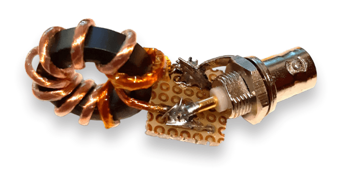
The probe in Figure 1 is designed to measure up to 50 A peak in a frequency range from 7 kHz to tens of MHz. The schematic in Figure 2 is quite simple: the wire whose current must be measured is passed through the toroid, which is an ordinary Amidon FT 82-43 core that performs well up to at least 50 MHz.
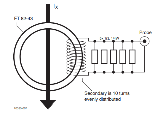
The secondary winding consists of ten turns of wire evenly distributed over the core. If available, use a medium-gauge stranded wire, but this is not mandatory. Due to the ratio of 1:10 turns, the maximum current in the secondary is 5 Ap.
The secondary side is loaded with 0.2 Ω, which was realized by a parallel connection of five 1 Ω resistors. At a peak current of 5 Ap, the peak voltage across these resistors is 1 Vp, which is very convenient for measurements with an oscilloscope. For a sinusoidal current, the average power dissipation at the resistors is R·I2 = R·Ip2 / 2 = 2.5 W or 0.5 W per resistor. A continuous sinusoidal current of 50 Ap can be measured only with 0.5 W or larger resistors. But, if the waveforms are pulsed or very short measurements are made, ¼ W resistors will do. That was my choice because I wanted to keep the design compact for better RF performance. OK, I also have to admit that these were the resistors I had on hand.
Usage
Figure 3 shows typical usage with a scope probe, using a BNC adapter for scopes. The device can also be used with a direct coaxial cable connection to the scope input, because 1 Vp is ideal for scope 1× operation: In this case, using a short cable is recommended to avoid reflections in the band of interest, because the coax will be mismatched on both sides. Even better, the coaxial cable can be terminated at its characteristic impedance on the scope side: Many modern scopes offer the ability to set the input impedance to 50 Ω, so this is particularly easy. In this specific case, one has to remember that the measurement will be slightly off-scaled, due to the parallel of the 50 Ω load with the 0.2 Ω incorporated in the probe (total resistance becomes 0.1992 Ω, giving a scaling factor of 50.2 A/V).
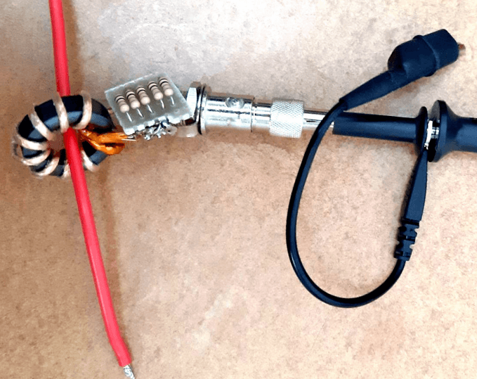
What must be avoided is attaching the scope probe directly to resistors using the clips and skipping the BNC connector, because when measuring high RF currents, even the minimum unshielded loop in the probes will add artifacts to the measurements.
Calculations
The design of the current transformer is not complicated, but some electromagnetic formulas are necessary. First, about the load resistor RL, which should be as small as practically possible in order to minimize the power loss introduced, because the circuit under measurement will “see” at least R·n2, where 1:n is the turns ratio (1:10) and R is the sum of RL (0.2 Ω) and of the secondary wire resistance (some mΩ). As already said, it is very important that the secondary side is evenly wound, as otherwise the circuit under test will present some stray inductance in series. On the other extreme, if we choose too low a value for RL, we’ll also have a very small voltage to measure, causing noise on the traces. Finally, RL should be greater than the secondary wire resistance.
In my case, I chose 0.2 Ω so that I could get 1 V at 5 A (50 A on the primary), which adds 2 mΩ to the circuit under test. The number of secondary turns, n, determines the current ratio. In case of a high-frequency CT, this number must be kept low to avoid self-resonance caused by stray capacitance together with high inductance. In the case of mains CTs, the frequency is quite low (50 or 60 Hz), and therefore n = 1000 is a common value. Powers of 10 are common, so that the current conversion ratio is simple, but other values are possible.
The highest usable frequency for a toroidal ferrite CT depends on the:
- performance of the ferrite material;
- self-resonance of secondary winding;
- resistor inductance (resistor itself and connections).
A design such as mine can easily work for up to several tens of MHz if a suitable ferrite, such as material 43 from Amidon/Fair-Rite, is used. High permeability cores used for EMI suppression can be used as well, but only up to much lower frequencies. Low permeability cores used for power chokes and high-Q inductors are not recommended, because their inductance per turn is too low, which affects the following point.
The choice of ferrite core also has an impact on the lowest usable frequency, for two reasons:
- In order to get good measurements, we’ll want the reactance of the secondary to be much greater than R, because it also acts as a load. Since reactance is X = 2π·f·L, this affects the lower frequency end. In practice, we’ll want X > 10·RL at the lower end.
- We must avoid saturation of the core, which happens at high current and low frequency. Saturation of ferrites happens for field B = 0.25…0.3 T, but in order to avoid nonlinear phenomena, we must stay below 0.2 T at the maximum current and minimum frequency.
For both reasons above, low usable frequencies with a small number of turns and a high current tend to require large cores. The key core parameters are AL, the inductance per turn, generally expressed in nH/n2 for RF cores, and the core cross-section S, which can be easily computed from core dimensions. In case of the Amidon FT 82-43 core, AL = 470 nH/n2 and the cross-section is 24.6 mm2 (easy to compute from outer diameter, inner diameter and height).
The inductance of 10 turns is therefore 470 nH x 102 = 47 µH (remember, inductance depends on n2). If we accept that X = 10·R ≈ 10·RL = 2 Ω, by reversing the reactance formula we get f > 6.8 kHz as the lower cutoff frequency. This may be acceptable or not, depending on the application, and a larger core, having a greater AL, will have a lower cutoff. In my case, for measuring a musical Tesla coil, I was interested in frequencies greater than 500 kHz, so this core was fine.
Regarding saturation, we have the fact that in the sinusoidal regime, the magnitude of field B (magnetic flux density) is abs(B) = Vp / (n·2π·f·S), where Vp is the peak voltage across the winding. This expression can be derived by equaling the two expressions of magnetic-linked flux Φc = L·I = n·B·S and replacing I with the absolute value of the AC magnetizing current abs(I) = V / (2π·f·L). If V and n are fixed in previous design phases, the only way of reaching a lower f is adopting a larger S, namely a larger toroid again.
In my case, Vp = 1 V, n = 10, S = 24.6 mm2 (pay attention to use correct units), so we have B < 0.2 T for f > 3.2 kHz, which is fine again, at least for my application. It may be confusing that current doesn’t appear in the calculation: actually, it is hidden behind V, because we know that 1 V corresponds to 50 A.
Improvements
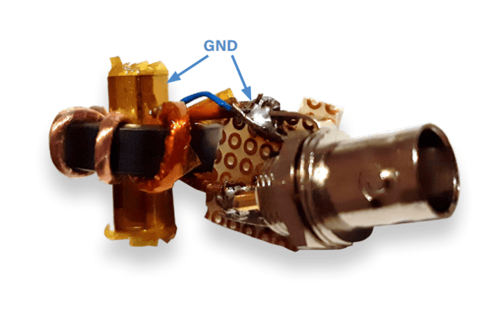
Capacitive coupling between primary and secondary windings can disturb measurements at the highest useful frequencies, or even at moderate frequencies if the primary conductor is subject to a high RF voltage.
The design can be improved by adding an electrostatic shield that avoids this capacitive coupling: In practice, the primary wire is passed inside a small piece of metal tube (typically copper or brass) connected to the output GND of the secondary, as shown in Figure 4. This doesn’t alter the magnetic linkage, but acts as an electric field blocker.
RF Current Transformer
This example of an RF current transformer together with the most important design criteria proves that this matter is less complex than it initially seems. I hope that the considerations and formulas presented here are useful in simplifying the handling of toroidal cores, as well as serving as a basis for your own developments.
About the Author
Roberto Visentin is a recently retired electronic engineer who worked on electronics and control systems for marine applications and underwater robotics. Still working as a freelance consultant, he enjoys finding more time to develop hobby projects in his home electronic laboratory.
Questions or Comments?
Do you have questions or comments about this article? Contact Elektor at editor@elektor.com.
This article originally appeared in Elektor May & June 2023. Become an Elektor member today!
Discussion (0 comments)