
Raspberry Pi Pico Makes an MSF-SDR
on
MSF is the UK’s equivalent of the German DCF77 time signal transmitter. This SDR project shows how a receiver and decoder for these (and other) time signals can be implemented quite simply and, above all, inexpensively. For the hardware you really won’t need much more than a low-cost Raspberry Pi Pico to receive, decode, and display MSF time signal information. In Germany the DCF77 transmitter in Mainflingen transmits an encoded long-wave time signal. Its equivalent based in the UK is the MSF signal formerly known as “The Rugby Clock.” It sends out time signals using a 60-kHz long-wave carrier signal. In the early days, it served as a frequency standard, and sent out a five-minute pulse train twice a day. The “transmission protocol” of the signal has changed several times over the decades, but it was not until 1977 that the encoding included time-of-day and date information that could be evaluated by the receiver.
The Project with Pico
Over the years, there have been many receiver/decoder circuits described in various Elektor articles that make use of the DCF77 signal, but this is probably the first time a design for an MSF receiver has been featured. There was, however, an add-on circuit for the good-old 6502 Junior Computer described in the English language edition of Elektor.
A lot of water has flowed under the bridge since then, and technology relating to receivers/decoders has progressed in leaps and bounds. In this article, we will use the latest “up-to-date” concepts to build a software-defined radio (SDR) using a small microcontroller board. The Raspberry Pi Pico board, which uses an RP2040 CPU clocked at 125 MHz (the in-house controller of the Raspberry Pi Foundation is equipped with dual 32-bit ARM Cortex M0+ cores), is a suitable, you could say, predestined piece of hardware for this application. Its analog-to-digital converter can run at 500 ksps. All this processing power can be purchased for an almost ridiculous €5. (See the Related Products below.)
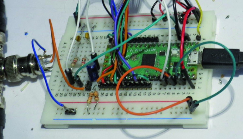
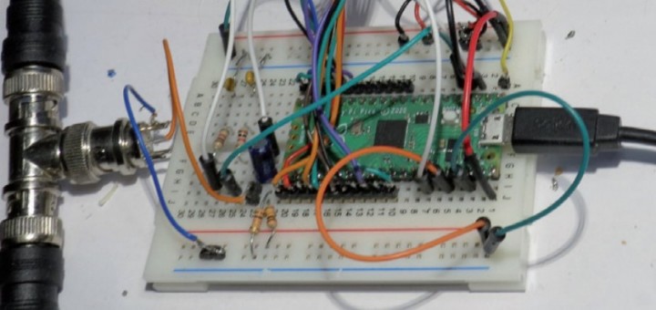
Here we show how to implement a complete receiver in hardware and software for the 60-kHz MSF time signal. The entire receiver, without a display but with an RS232 output and antenna connection, is shown in Figure 1.
Hardware
First, we will take a look at the hardware necessary to build the SDR. There are just a few additional items to connect to our pico board.
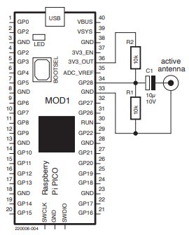
Antenna Input: We use the analog input pin ADC2 (GPIO28, on the Pico board pin 34) to receive signals from the antenna. The ADC uses the internal 3.3 V as a reference voltage. This pin must therefore be biased at half the reference voltage. The two resistors in Figure 2 take care of this. The 10-µF capacitor C1 provides AC coupling for the incoming signal.
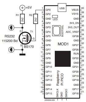
RS232 Output: In its simplest form (without an LC display), the receiver uses a serial interface (115,200 Bit/s) to output the data. The interface is implemented by the circuit shown in Figure 3. We cannot use the USB port to output the serial data because it would generate interrupts to our software in an unpredictable way.
PWM DACs: When no LC display is connected, it is possible to use the DACs with pulse width modulated (PWM) signals to create an easy aid for debugging. We have set up two PWM DACs with the associated low-pass filters as shown in Figure 4.
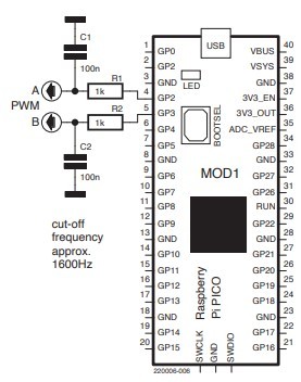
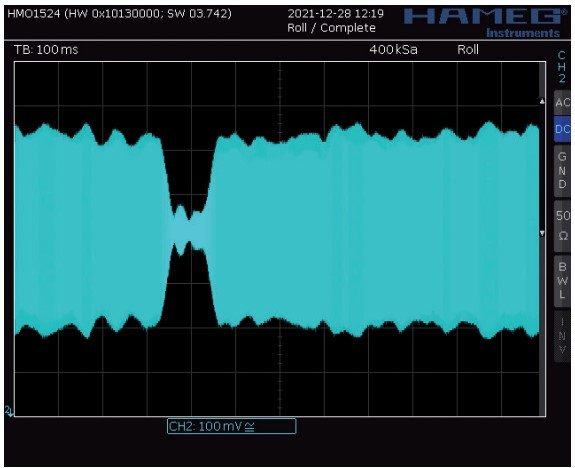
Using GPIO 2 and GPIO 3 as PWM outputs, for example, the demodulated signal and Bit-Timer signals can be displayed on a scope (Figure 5).
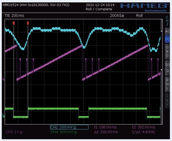
the SecondTimer showing Sampling trigger pulses and below is the digital sigValue signal.
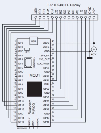
LCD: The 3.5-inch Arduino 8-bit module ILI9486 (non touch screen version SKU MAR3502 [4]) can be used as the LCD. This 3.5-inch Arduino shield has 480x320 coloured pixels and retails for around €10. Its connection to the Raspberry Pi Pico is shown in Figure 6.
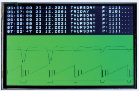
The received signal is shown on the LCD together with a waveform showing bit timing information. The received time information is shown in plain text above the waveform (Figure 7). If you do not need to display this information you can choose to simply omit the LCD without the need to make any changes to the software.
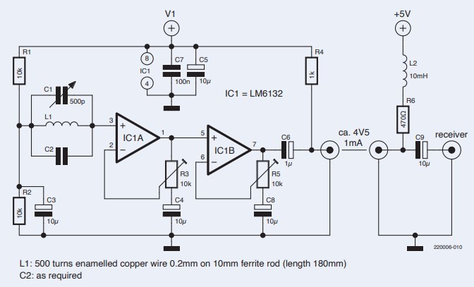
Active Antenna: We have already covered the antenna connection; the circuit of the active antenna can be seen in Figure 8. It is essentially based on the LM6132 dual operational amplifier. This op-amp is particularly suited for this application with an operating voltage of 2.7 to 24 V, 10 MHz gain bandwidth product, rail-to-rail input and output signal capability and low current consumption of 360 µA per amplifier. No doubt other op-amps would also work here but if you intend to replace the LM6132, check carefully whether it will match the spec.
Programming the Input Mixer
After the hardware, we come to the programming. The analogue paths of the SDR is structured as shown in Figure 9. The Raspberry Pi Pico can be programmed using several different languages. For this application we chose C using the Microsoft Visual Studio Code development environment running on a PC under Windows 10. Let’s look at how the different parts function.
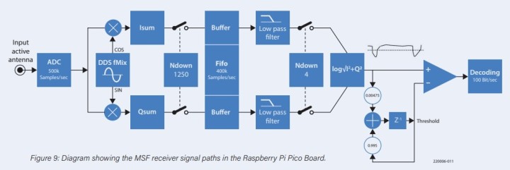
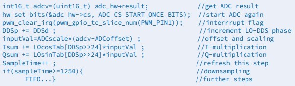
The ADC Sample Routine is triggered by the PWM and called 500,000 times per second via interrupt. The Offset ADCoffset = 2048 is subtracted from the ADC value and the result is then multiplied by ADCscale = 10 (Listing 1).
The local oscillator (LO-DDS) phase is updated and the input value is multiplied by the cosine (in-phase or I signal) and the sine (quadrature-phase or Q signal). The products are summed over 1250 samples (in Isum and Qsum). The values are then (in Listing 2) passed to a FIFO for further processing, which then takes place at 500000/s/1250 = 400 samples/s. This sample rate is so low that all the further processing can be carried out using double variable values.
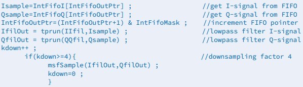
The values are read from the FIFO and passed through a fourth-order Butterworth low-pass filter with a cut-off frequency of 3 Hz. During development it was found that this low cut-off frequency was necessary because the author’s antenna received strong interference signals directly adjacent to the wanted signal. This is followed by another down-sampling, this time by a factor of 4, so that 100 samples/s are then processed.
The msfSample() routine in Listing 3 then calculates the carrier amplitude ampl from the I/Q components. The logarithm of ampl is derived and in turn stored in ampl which makes it easier to decode the bits.
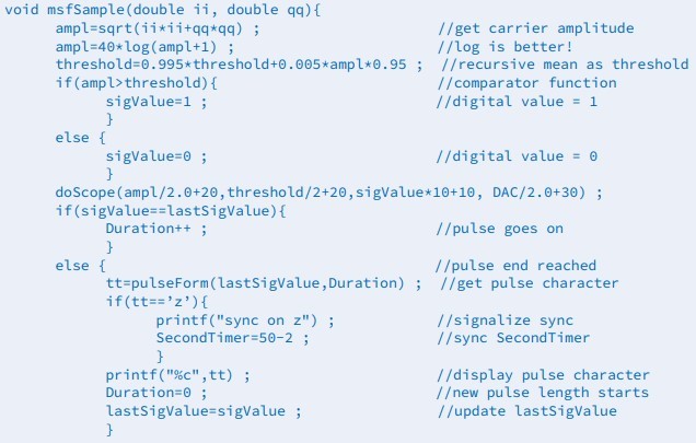
The switching level threshold is derived from ampl via a first-order recursive filter calculation. The signal ampl is then compared with the switching level threshold to determine its digital receive value sigValue. Now with the analogue signal processing covered we can look at how the data is recovered from the received signal and how this corresponds to the time-of-day information.
Reading the Bits
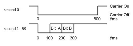
The MSF transmitter sends out RF carrier pulses at each second as shown in Figure 10. At second 0 of every minute the carrier switches off for 500 ms. The SDR uses this pulse for synchronization. The pulses emitted at each of the following 59 seconds contain two bits of information: A and B. At the start of each of these seconds the carrier is off for 100 ms (corresponding to 10 samples in our application). If Bit A = 1, the carrier remains off for a further 100 ms, and if Bit B = 1, the carrier is off for another 100 ms.
In SecondTimer, a timer, synchronised to each second, runs from 0 to 99. The software decoding works as follows: In Duration, the pulse length of the current pulse is measured. If a 0.5 s absence of the carrier is detected, SecondTimer is set to the value 50-2 = 48 so that the SecondTimer timer now runs synchronously with the second (Listing 4). At the same time, the minute is synchronized by setting the value of the current second to 0 in doMinuteSync().
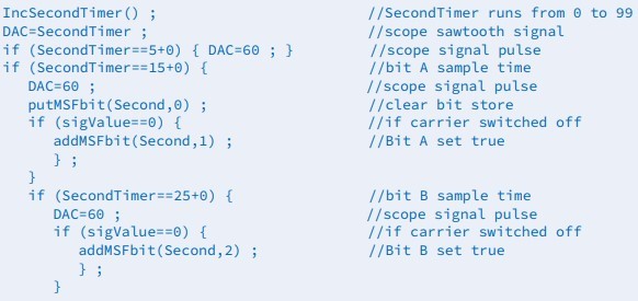
With the help of SecondTimer, the received signal is sampled at the mid-bit position of Bit A and Bit B (SecondTimer==15 and SecondTimer==25) in order to determine the values of these transmitted bits. We simply output the received digital value via GPIO-Pin 4 (Pico-Pin 6):
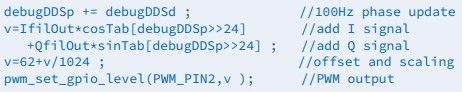
gpio_put(GPIO4, sigValue); // Output sigValue at pico GPIO4=pin 6
The value of SecondTimer is also output later for debugging purposes via PWM, as are the values of ampl and DAC. This is achieved with the following two statements:
pwm_set_gpio_level(PWM_PIN1, ampl/5.0 ); // Output amplitude
pwm_set_gpio_level(PWM_PIN2, DAC ); // Output timing
Decoding Time Information
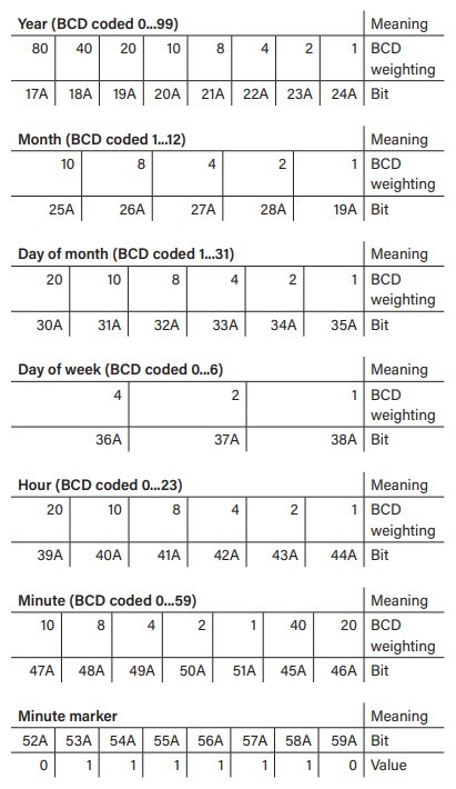
Whenever SecondTimer is synchronized by the 0.5 s gap, one minute has passed and we can evaluate the latest time information. The received data bits are in the values MSFbits[0 to 59]. The transmitter encodes the information listed in Figure 11 into these bits.
The time and date information is then simply reconstructed as in Listing 5 to give hours and minutes.
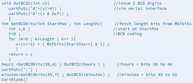
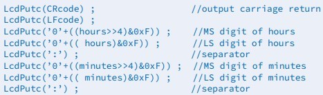
We also display the same information that we send out via the serial interface as text on the LCD. This is done using the instructions given in Listing 6.
A parity check on the received information is evaluated as in Listing 7. The monitored bits are the A-bits of the transmitted information. The four check bits are B-bits of each corresponding seconds pulse. Four parity checks are carried out, the integrity of up to 12 bits are protected by one parity bit.
Debug Signals
Classic superhet receiver designs mix the incoming RF signal with a variable frequency local oscillator signal to produce a lower intermediate frequency or IF. The IF signal is then filtered with a relatively narrow band filter. The IF signal of the MSF60 receiver can also be viewed using an oscilloscope. Our receiver mixes the input signal down to IF = 0 Hz. If you want to observe an AC IF signal, you can upconvert the 0 IF signal to an AC IF. The circuit block diagram is shown in Figure 12.
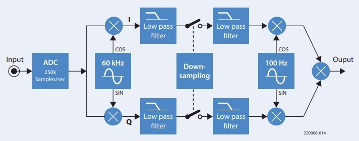
The software to perform the necessary upmixing is shown in Listing 8.
A PWM output is used as the DAC. The 100 Hz AM-modulated IF signal is shown in Figure 13.
This completes the design and construction of the MSF receiver. Only one core of the processor is used in this application, leaving plenty of computing power for expansion. The bit decoding, for example, could be made more error-tolerant. A DCF77 receiver could be built in much the same way, only the bit decoding process would need to be adapted. The MSF signal reception here in Aachen (Germany) is much weaker than the DCF77 signal with an equivalent SDR. This often results in parity bits indicating errors in the received information but sufficient error-free messages still get through frequently enough to allow accurate time of day information to be displayed reliably.
Working with an RP2040
We have shown that with very little additional hardware, the Raspberry Pi Pico board can be turned into a complete MSF SDR. The most complex element of this build is construction of the active antenna. Given the processing power and low cost of the board this application shows what even a hobbyist with few resources can achieve nowadays. You often read how easy the Pico board can be programmed in Python, but in this application, it will not be able to cope with the 500k sample rate of the input signal. With C, however, the microcontroller hardware can be addressed more directly and programmed efficiently. We see here that even without the benefit of a floating point unit (FPU) the RP2040 is still more than capable of implementing a low-pass digital filter.
Questions or Comments?
If you have any technical questions regarding this article you can contact the author at ossmann@fh-aachen.de or the Elektor team at editor@elektor.com.
More on the Raspberry Pi Pico
Check out this Elektor video about the Raspberry Pi Pico!
Discussion (7 comments)