Plunging oil prices – US Tight Oil Boom or Bust?

The global shale oil and gas industry is still in its infancy (in the learning curve) but the United States industry is far ahead and has shown inspiring results as their shale/tight oil production increased from 1.24 million barrels daily (MMBD) in 2007 to 4.68 MMBD in 2014 – which represents approximately a 3-3/4 fold increase [1].

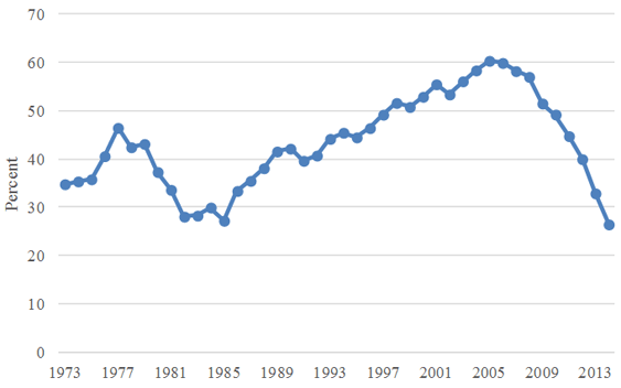
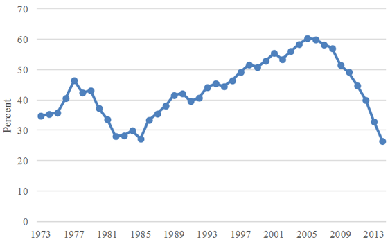
This increase in oil production was supported by sustained higher oil prices of over $100/BBL that provided a breathing space to the industry, allowing it to develop and master innovative technology (horizontal drilling, hydraulic fracturing, multi fracturing, less use of water etc) and was well supported by favorable policies of various States. The sustained higher oil prices encouraged a shale gas boom in the US that also produces substantial condensate. Even in the regime of very low Henry Hub (HH) prices, we saw tremendous growth in US gas production – resulting in reduced gas imports from Canada. The combined effect of both these and other factors allowed the US to reduce its net oil import dependency from 60% in 2005 to below 27% in 2014, despite the growth in domestic oil demand that was hovering around 18 MMBD recently. (Figure-1).

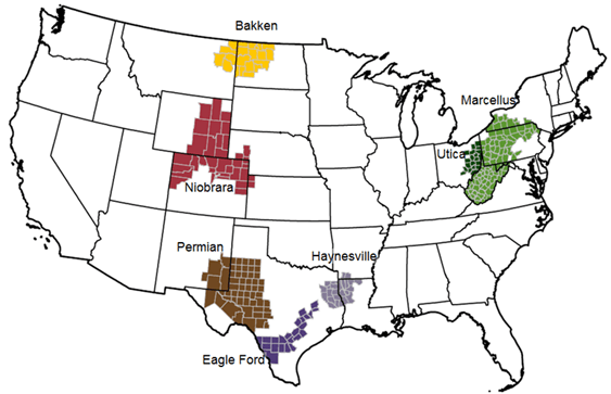
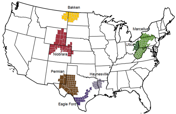
The question is how will the collapsing oil prices from over $95/BBL during the period of March 2011-October 2014, to below $45/BBL that now hovers around mid fifties affect the US tight oil industry? Do we expect a continued boom in the US tight oil production or is a burst immanent? One possible outcome is that lower oil prices result in cutting back drilling activities that in turn would reduce US tight oil production with some lags. The reason being that tight oil/gas is expensive to develop/produce and the production decline rate is significantly higher compared to conventional oil. Therefore, in order to sustain the level of production more wells need to be drilled and fractured. However, thus far, this has not been the case in the face of plunging oil prices, US tight oil production is still increasing, even after a number of months of sustained lower oil prices and decline of the drilling rig count. This paper reviews and explores each of the seven tight oil plays – Bakken, Eagle Ford, Haynesville, Marcellus, Niobrara, Permian and Utica (see Map-1) [2]. It looks at how the production from these prospects will help the country in reducing oil import dependency and why tight oil production is insensitive to oil prices and rig count. The analysis is both qualitative and quantitative using econometric modeling.

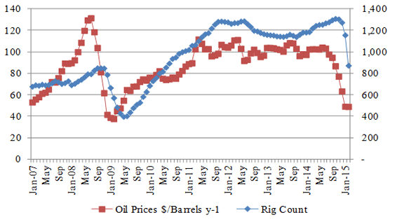
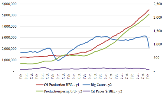
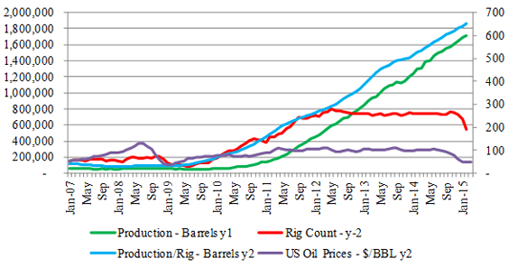
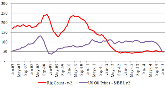
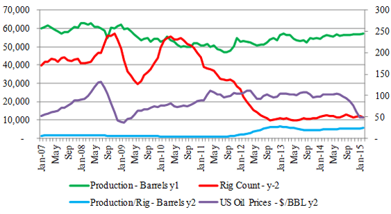
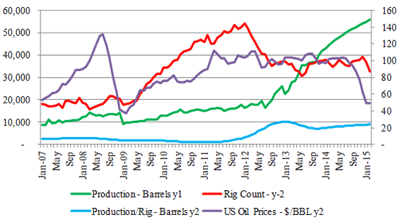
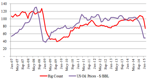
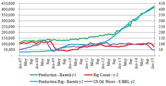
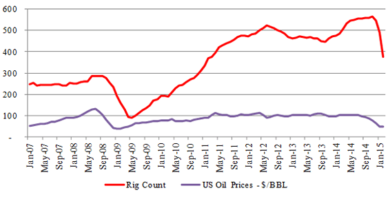
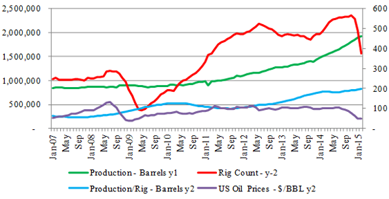
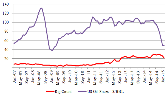
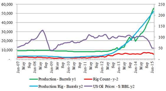
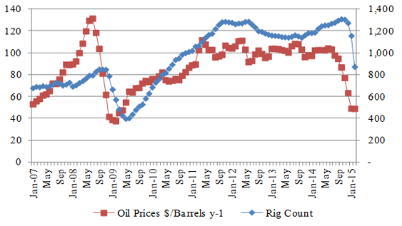
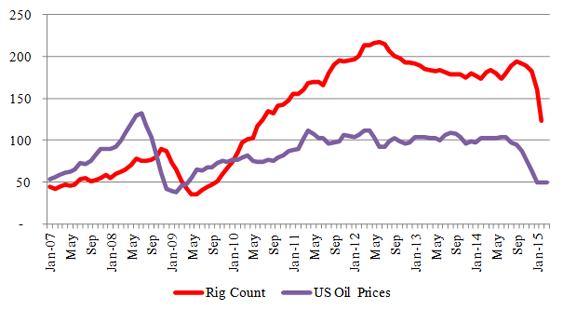
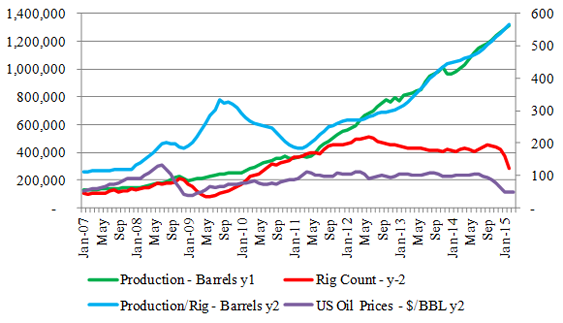
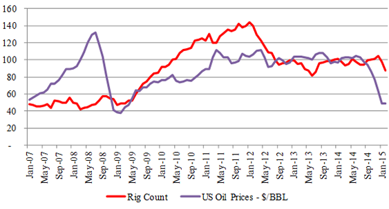
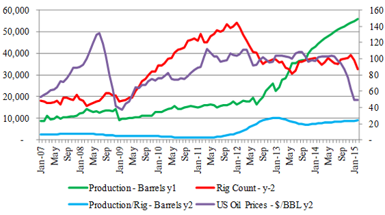
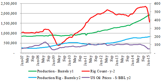
Figure-2 [3] illustrates the US total tight oil profile. The burgeoning oil prices during 2007/2008 set the momentum of US tight oil boom. The higher oil price expectations allowed breathing space to the oil and gas industry in exploitation of unconventional resources that are more abundant than conventional. During the early period, generally daily productivity per well was quite low and hence so was the production level. But drilling of thousands of wells allowed a deeper understanding of the geological prospects and technology in carrying out hydraulic fracturing more efficiently – improving productivity per well. As a result of higher oil prices, horizontal drilling and hydraulic fracturing, tight oil production increased from 1.24 MMBD in 2007 to over 4.68 MMBD at the end of 2014. Visual inspection of these trends demonstrates that there is a positive correlation between the number of rig count and oil prices with some lags. However, both oil production and daily production per rig seems to be insensitive to both oil prices and rig count. The aggregating of data for the seven different prospects could be providing a biased assessment, therefore it is imperative to analyze the individual prospects to determine whether the similarities and divergences exist across the prospects. And if so why.

United States Tight Oil Behavior

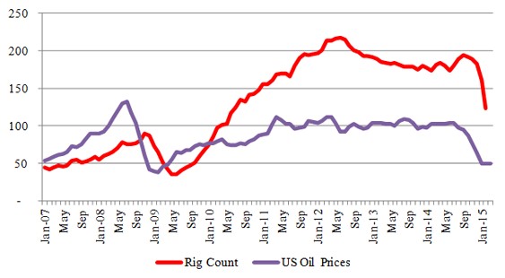
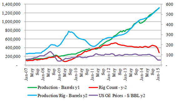
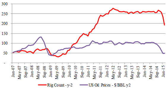
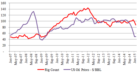
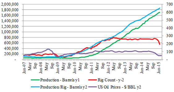
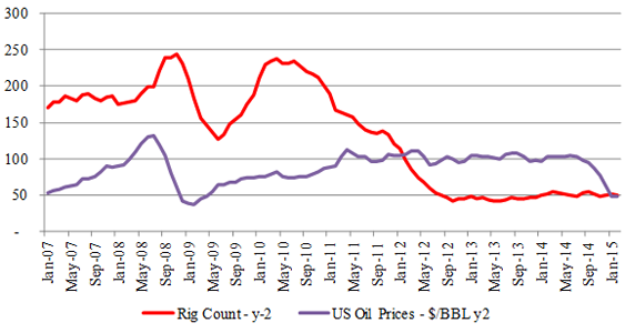
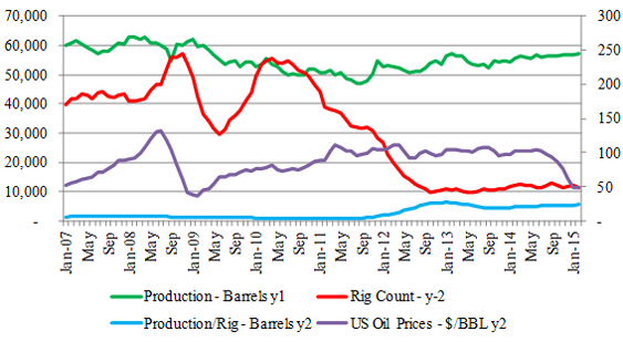
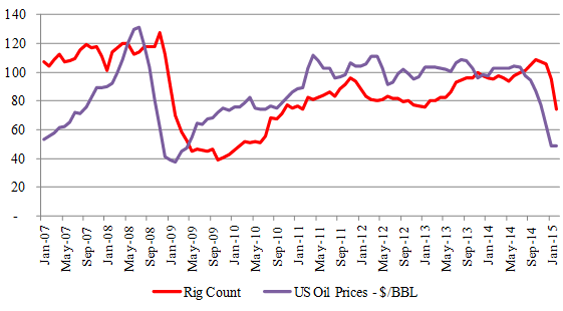
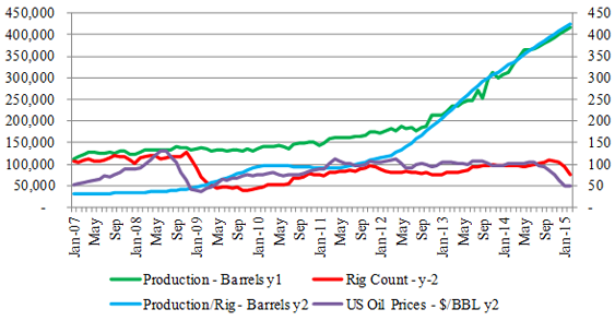
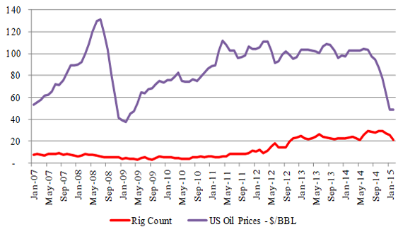
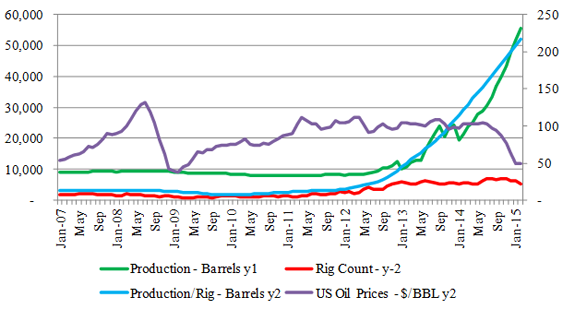
Figures-3 to 9 illustrate the relationship of oil prices, rig count, production and productivity per well (daily barrel production per rig) for each of the seven plays. Visual inspection of these trends generally demonstrates that all the seven prospects - Bakken, Eagle Ford, Haynesville, Marcellus, Niobrara, Permian and Utica show similarities (Figure-3-9 (a)). Generally, all seven prospects demonstrate a positive correlation between oil prices and rig count, though magnitude and number of lags differs from prospect to prospect. This could be due to different cost structures that vary between prospects, to differences in geological conditions, the extent of difficulty, extent of available infrastructure, proximity to market, etc. For example, some wells are significantly deeper than others thus more costly to drill and complete. In addition, the period of contracts with service companies also vary, therefore the response to increase/decrease in rig counts to increase/decrease in oil prices differ.

Another interesting feature of these trends is highlighted in Figures-3-9 (b). With the exception of Haynesville to some extent, oil production and productivity per rig did not respond to either oil prices, or the number of rig count. In fact, collapsing oil prices did not deter aggressive upward movement in oil production even after several months had elapsed. The question is what causes this to happen? Is it that the break-even prices have substantially declined or can we expect a burst soon, or something else?

One explanation is certainly related to the industry learning curve. That is drilling and hydraulic fracturing of thousands of wells allowed them to better understand the geology, optimum number of fractured spaces required to maximize production, less use of water for hydraulic fracturing which may have helped them to cut costs. Yet another explanation could be related to the difference between drilling strategies for unconventional and conventional resources. The strategy of unconventional resources is driven by economics (profitability of individual wells) rather than maximizing the overall resources recovery. Therefore the biggest challenge in the case of unconventional resources is not to find the productive zones, but rather to find zones that are most conductive to effective stimulation. As a result of this strategy, they often select the potential fracture treatment parameters that produce profitable wells, but leave behind considerable hydrocarbon resources.

Therefore, when oil prices tumbled production and productivity per rig kept increasing, this may have been due to revisiting these reserves that were not fractured earlier during the regime of higher oil prices. Revisiting and fracking of these reserves previously left behind probably helped the industry to continue to increase production as this does not require additional drilling of wells. Thus production continues to move upwards, despite a decline in rig count and oil prices. The question is how long this phenomenon will last. This is difficult to predict in the absence of historical data, however some of these unusual trends will become visible during the next few months if oil prices remain around $50/BBL. If oil production increase continues even after several months have passed then this could be due to the combination of revisiting untapped reservoirs to frack and declining break-even costs to below $50/BBL for some prospects. If this is the case it would be alarming for OPEC, who are trying to increase/maintain their market share and are therefore refusing to cut oil production. Should Iranian sanctions be lifted and if the US Congress waives export restrictions, it will be a dilemma for OPEC members how to compromise between market share and balance their ever rising budgetary requirements.

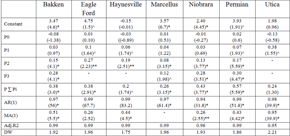
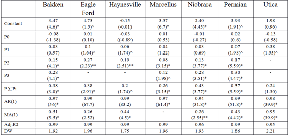
Visual inspection reveals that there is a positive correlation between rig count and oil prices, but there seems to be no correlation between oil production, rig count and oil prices. Table-1 depicts the estimated results for each of the seven plays. In each of the prospects, rig count is run against oil prices and monthly oil production also tested against oil prices using monthly data for the period January 2007 to February 2015. Visual inspection of the graphs has established there is lag structure present. We have used polynomial distributed lag models with varying weights and lag structure. The best estimated results are reported here.

As was expected the rig count did not increase/decrease in response to increase/decrease in oil prices instantaneously, rather it took a number of months before the full impact of one percent increase/decrease in oil price affected the rig count. Generally the data shows that the response during the first two periods was either statistically insignificant or marginal; however, it strengthened with time and full impact was witnessed after a lag of four periods. The short-term elasticity is generally insignificant while the full strength was established in the long-run when one percent increase/decrease in oil prices lead to increase/decrease in rig count between 0.2% for Haynesville and 0.57% for Permian. More than 99% of the variation in rig count is explained by oil prices. When monthly oil production is run against rig count and oil prices in all the cases models were suffering from an autocorrelation problem and the given explanatory variables were also statistically insignificant.

Conclusions

What we have learned from history is that our oil and gas industry is quite dynamic and adjusts quickly in challenging situations which is supported by innovative technology. In any given situation oil production and more particularly tight oil production should be responsive to changes in oil prices and rig count. However, the contrary seems to be the case, despite decreasing rig count and oil prices, US tight production kept rising in almost all seven plays. Normally a lag of few months occurs before a response to changes in oil prices can be observed, however, generally tight oil production aggressively moves upward. This may be due to a number of factors – decrease in break-even cost and revisiting and fracturing leftover reserves from the period of higher oil prices. The US tight oil industry would be clearly a winner if they sustain their current level of production with oil price of mid-fifties during the rest of the year. So far it appears that US tight oil industry successfully weathers this episode of lower oil prices. Having said that, the next few months will be critical to determine whether the US tight oil industry continues to boom or will burst in response to lower oil prices.


1. The US industry uses the term tight oil production instead of shale oil because it is a more encompassing term with respect to the different geologic formations producing oil at any particular well. Tight oil is produced from low-permeability sandstones, carbonates (e.g., limestone), and shale formations.
2. While shale resources and production are found in many U.S. regions, this paper is focusing on the seven most prolific areas, which are located in the Lower 48 states. These seven regions accounted for 95% of domestic oil production growth and all domestic natural gas production growth during 2011-13.
3. Source for Figures 2 to 9 – Energy Information Administration (EIA) web-site data base.


Dr. Ghouri is Senior Performance Analyst in Finance and Planning directorate. The views, findings, interpretations, and conclusions expressed in this paper do not necessarily reflect the views of Qatar Petroleum.
Dr. Ansari is a general dentist in private practice in Qatar, with an original background of statistics and economics

Image: USGS