
Understanding the Neurons in Neural Networks (Part 1): Artificial Neurons
on
Artificial intelligence (AI) and machine learning ( ML ) are two of the industry's hottest topics. Thanks to successes covered in the press, with AI beating the world's best Go players [ 1 ], and failures, such as autonomous vehicle accidents [ 2], AI has become part of the lingua franca. While AI and ML have been democratized thanks to cloud-based tools such as TensorFlow, these huge powerful platforms can seem intangible if you are trying to understand how ML works "under the hood." In this series on neural networks, we go back to basics and explore most of these systems' basic building block. Along the way, there are plenty of examples to try, cases of cool and obscure ML projects, and at the end, we'll even bestow an Arduino with a brain. Let's dive into the exciting subject of neural networks.
Computing Challenges
AI and ML are “the” computing challenges of our time. AI, which focuses on using computers to mimic human intelligence, and ML, which targets pattern recognition of structured and semi-structured data, commands significant annual investment from research projects to the development of semiconductor technology and computing platforms. And, thanks to “the cloud,” the technology is easily accessible to those wanting to explore and test their ideas.
But what are neural networks? How do all these clever algorithms work? How do they learn? What are their limitations? And is it possible to play around with the nuts'n'bolts of ML without registering for yet another cloud service? These are precisely the questions that this short series on neural networks will address in four parts:
- Part 1 — Artificial Neurons: In the first part of this series on neural networks, we start by going back to the 1950s to look at the early research to develop an artificial neuron. From there, we quickly move to a multilayer perceptron (MLP) software implementation that uses backpropagation to “learn.”
- Part 2 — Logical Neurons: one of the challenges with early neurons was their inability to solve the XOR function. We examine if our MLP can solve this problem and visualize how the neuron learns.
- Part 3 — Practical Neurons: We apply our MLP to part of the autonomous driving problem: recognizing the state of traffic lights using a PC-based program.
- Part 4 — Embedded Neurons: We wrap up the series on neural networks by focusing on embedded neurons. If it works on a PC, it should work on a microcontroller, shouldn’t it? Using an Arduino and an RGB sensor, we detect traffic light colors once more.
Lazy Learning
Learning is hard work for humans and also for AI it seems. Research undertaken by the TU Berlin, Fraunhofer HHI, and SUTD made AI systems explain their decision-making strategies [13]. The results were eye-opening. While the AIs all performed their tasks admirably, they displayed breathtaking cheekiness in their decision-making corner-cutting. One algorithm correctly determined the presence of a ship in an image but based the decision upon the fact there was water in the photo. Another correctly detected images were containing horses but based its decision upon a copyright mark in some images, rather than learning the visual attributes of a horse.
Neural Networks: A Little Neuron History
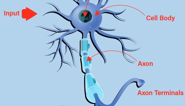
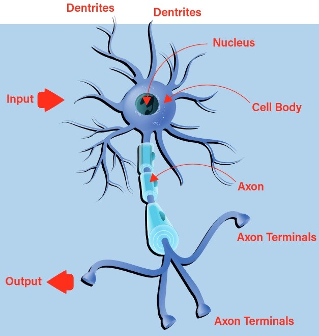
Early attempts at building a digital, or artificial, neuron turned to nature for inspiration. The biological neuron accepts inputs via its dendrites and passes on any resultant output through its axon to the axon terminals (Figure 1). The decision of whether to emit a stimulus via the output, known as the neuron firing, is undertaken using a process called activation. Should the inputs conform to a learned pattern, the neuron fires. Otherwise, it does not. It can quickly be seen that, with chains of interconnected biological neurons, very complex patterns can be recognized.
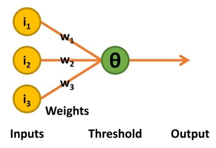
The first artificial neurons developed were McCulloch-Pitts networks, also known as Threshold Logic Units (TLU). These were simple “decision machines” capable of replicating the function of logic gates. They accepted and output only logical values of 0 and 1. To implement their pattern recognition capability, weight values would need to be determined for each input, either mathematically or heuristically. Sometimes an additional input would be required too (Figure 2, AND and OR functions).
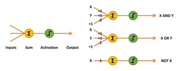
Figure 2: McCulloch-Pitts network sums the inputs multiplied by their weights, activating an output of 1 if the result is equal to or greater than 0.
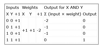
The inputs to the network are simply multiplied by their weights and summed together. The decision to output a 1, or activate, is implemented using a linear threshold unit. Should the result be equal or greater than 0, a 1 is output. Otherwise, the output is 0 (Table 1).
Perceptrons
The next stage of development came in the 1950s with work undertaken by psychologist Frank Rosenblatt [3]. His perceptron retained the binary inputs and linear threshold unit decision-making of the McCulloch-Pitts TLU. Thus, the output was also a binary value of 0 or 1. It differed, however, in two distinct ways: the threshold level (known as theta, Θ) for deciding on the output value was adjustable, and it supported a limited form of learning (Figure 3).
and used an iterative learning process.
The learning process functions as follows: the perceptron outputs a value of 1 only if the sum of the product of the inputs and weights is greater than theta. If the output with respect to the combination of inputs is correct, nothing is changed.
Should a value of 1 be output when a 0 is required, theta’s threshold level is increased by one. Additionally, all weights associated with inputs of 1 are reduced by 1. Should the opposite occur, i.e. a value of 0 is output when a 1 is required, all weights associated with inputs of 1 are increased by 1.
The thinking behind this process is that only the inputs with a value of 1 can contribute to an unwanted output of 1, so it makes sense to reduce their impact by reducing their corresponding weights. Inversely, only inputs with a value of 1 can contribute to the desired output of 1. If the output is 0, and not 1 as desired, the associated weights must be increased.
In 1958, the “Mark I perceptron” was built as a hardware implementation, having first been implemented in software on an IBM 704 [4]. Connected to 400 cadmium sulfide photocells that formed a rudimentary camera and using motors connected to potentiometers to update the weights during learning, it could recognize the shape “triangle” once trained [5].
The Trouble with Perceptrons
While this heralded in a new era where an electronic system could potentially learn, there was a key issue with this design: it could only solve linearly separable problems. Going back to the earlier McCulloch-Pitts TLU, the simple AND, OR, NOT, and the NAND and NOR functions are all linearly separable. This means that a single line can split the desired outputs (with respect to the inputs) from the undesired outputs (Figure 4). XOR (and the complementary XNOR) functions are different. When the inputs are the same (00 or 11), the output is 0, but when the inputs are different (01 or 10), the output is 1. This requires that the desired output is classified into a group with respect to the inputs. Put simply, the perceptron cannot be trained to learn how XOR or XNOR works or replicate its function.
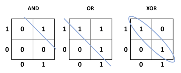
be linearly separated, using a straight line, from the 0 output states. For XOR, the 1 output
states cannot be linearly separated from the 0 output states, and is something a
perceptron cannot learn.
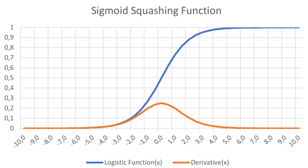
The other key issue lay with the activation function used. The linear threshold unit made a sharp jump between being inactive and active. Research that resulted in the Delta Rule [6] network showed that gradient descent learning was a crucial element in the neural network learning process. This also meant that any activation function must be differentiable. The sudden jump from 0 to 1 in the linear threshold unit is not differentiable at the transition point (slope becomes infinity), and the remainder of the function simply delivers 0 (output remains unchanged).
It was proposed that a multilayer network that resulted in one or more hidden nodes between the input and output nodes would solve the XOR problem. Furthermore, a differentiable function, such as the logistic function (Figure 5), a sigmoid curve, could provide a smooth activation function that supported gradient descent learning. The big challenge was the learning – how would all the weights be trained?
with gradient descent learning in neural networks.
The Delta Rule approach had shown that, by calculating the error squared of the network (desired output – actual output) and implementing a learning rate, the weights in the network could be successively improved until the optimal set of weight vectors had been found (Figure 6). The addition of a layer of hidden nodes between the input and output made this more complicated to calculate, but not impossible, as we shall see.
two output nodes. The hidden and output nodes can use a sigmoid curve to
determine their output in the feedforward phase.
Multilayer Perceptron
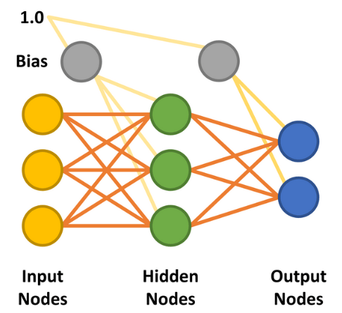
With the hidden layer added, the multilayer perceptron (MLP) was made possible. The simplest form of MLP neural network makes use of a single hidden layer. All the nodes are linked (known as ‘fully connected’) with weights assigned between each input and hidden node and between each hidden and output node (Figure 7). The lines between the nodes represent the weights. The desired inputs are applied to the input nodes (values between 0.0 and 1.0), and the network calculates each hidden and output node’s response — a step known as the feedforward phase. This should deliver a result indicating that the input values match an output category the network has learned.
For example, the inputs could be linked to a 28 × 28 pixel camera pointed at handwritten numbers. The MNIST database of handwritten digits containing just such image sizes could form the training set [7]. Each of the outputs would represent one of the numbers from 0 to 9. With the number 7 held in front of the camera, each output would report the input’s likelihood of being its value. Output 0 will, hopefully, indicate that the handwritten number is unlikely to be a 0, as should eight other outputs. But output 7 should indicate a high likelihood of the handwritten number being 7. Once trained, this should be the expected functionality for a 7 from the training data set or a newly handwritten 7 recognizable by a human.
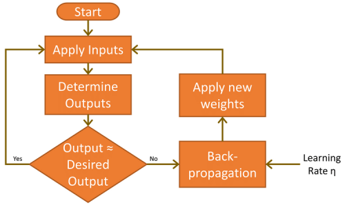
Before this can happen, the network needs to learn the task at hand. This is achieved by applying the input (handwritten 7s) and analyzing the results the outputs deliver. As they are initially unlikely to be correct, a learning cycle is executed to modify the weights such that the error is reduced. This iterative learning process, known as backpropagation, is executed many thousands of times until the network’s accuracy meets the application’s demands. In the world of ML, this is termed "supervised learning."
There are two further important factors to consider in the feedforward and backpropagation phases. The first is bias. A bias value of 1.0 multiplied by a weight (between 0.0 and 1.0) is applied to the hidden and output layer nodes during the feedforward phase. Its role is to improve the network’s capacity to solve problems and, in essence, pushes the logistic activation function (refer again to Figure 5) left or right. The other value is the learning rate, again a value between 0.0 and 1.0. As the name implies, this determines how quickly the MLP learns to solve the problem given, also known as the speed of convergence. Set too low, the network may never solve the problem to a suitably high level of accuracy. Set too high, it runs the risk of oscillating during learning and also not delivering an accurate enough result (see also “Limitations of gradient learning”).
The MLP described here could be considered a “vanilla” design. Neural networks can, however, be implemented in a multitude of ways. These include having more than one hidden layer, not fully connecting the nodes, linking later nodes to earlier nodes, and using different activation functions [8].
Neural Networks: Limitations of Gradient Learning
There are times when the neural network is seemingly incapable of learning, despite having previously learned the required functionality with the same node configuration. This may be due to the network getting stuck in a "local minimum" instead of finding a ‘global minimum’ of the error function.
MLP in Action
With the principle hopefully clear, we will now examine a concrete example. It follows an excellent article by Matt Mazur, who took significant time to explain backpropagation in an MLP with a single hidden layer [9]. Our review here will be at a high level, but those interested (and not afraid of mathematics) are advised to study Matt’s piece for more detail. Once the mathematical principle of operation is covered, we will review a software MLP implementation that will operate using the same parameters used for this theoretical analysis. If you are interested in following along, there is an Excel spreadsheet that matches Matt’s worked example. Simply download or clone the repository from GitHub [10] and take a look at workedexample/Matt Mazur Example.xlsx in the folder.
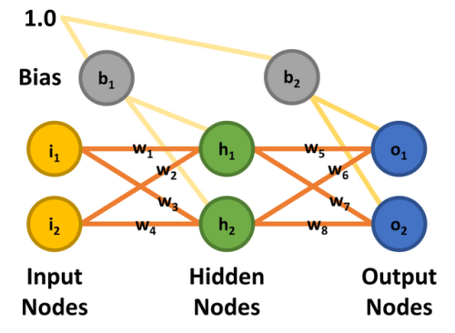
To keep things simple, a two-input, two-output MLP with two hidden nodes is used. The input nodes are labeled i1 and i2, the hidden nodes h1 and h2, and the output nodes o1 and o2. For this exercise, the aim is to train the network to output 0.01 on node o1 and 0.99 on o2 when node i1 is 0.05 and i2 is 0.10. There are eight weights (w1 through w8) and two bias values (b1 and b2). So that the math can be replicated, all input nodes, biases, and weights are assigned the values shown in Figure 8 and match with Matt Mazur’s article.
Feedforward
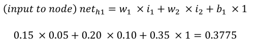
The feedforward phase to calculate the outputs o1 and o2 functions as follows. Each hidden node receives an input that is the net sum of the inputs multiplied by the weights, plus the bias input (b1 = 0.35). Using the process and equations provided by Matt Mazur, the input to h1 is the sum of i1 multiplied by w1 (0.15), i2 multiplied by w2 (0.20) and b1 (0.35).
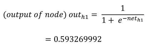
Each hidden node’s output value is determined by the logistic (activation) function, squashing the hidden node’s output to between 0.0 and 1.0. This is calculated as follows:
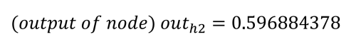
Repeating the process for h2 (with w3 = 0.25, w4 = 0.3, and b1 = 0.35) we get:
The net inputs to the output nodes are calculated in the same manner, using the calculated output values from the hidden nodes and applying the weights 5 through 8 (w5 = 0.4, w6 = 0.45, w7 = 0.5, and w8 = 0.55) and the bias value b2 = 0.60.
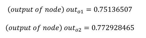
As already stated, our goal is to get o1 to output 0.01 and o2 to output 0.99, but we can see that we are some way off from this result. The next step is to calculate the error in each output using the squared error function, as well as the total error as follows:
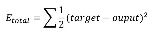
This is calculated for each output as follows:
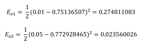
Finally, the total error for the network can be established:
The next step is to figure out how to improve on this error.
Backpropagation
Backpropagation is where the “learning” happens. The process here involves determining the contribution each weight has on the total error. It starts by looking at the weights between the hidden nodes and the output nodes. What complicates matters is that w5 contributes to the total error through two output nodes, o1 and o2, that are also influenced by the weights w6 through w8. It should also be noted that the bias values play no role in these calculations.
The math required to define this is quite complex, but it reduces to some simple multiplications, additions, and subtractions. Calculating the new value for w5 while factoring in the chosen learning rate, η (0.5), is performed as follows:
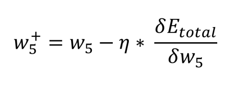
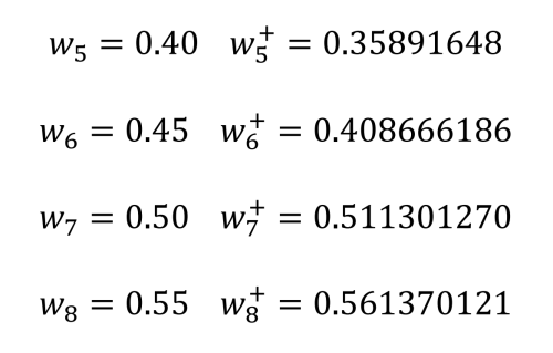
From this, we can review the old weights and compare them with the new weights for w5 through w8:
Applying a quick sanity check, we can see this makes sense. We want o1 to be pushed down by w5 and w6 towards 0.01, and o2 to be pushed up towards 0.99 by w7 and w8.
The final step is to determine the contribution the weights between the inputs and the hidden nodes have on the error at the output. As before, the math reduces to simple multiplications, additions, and subtractions. In fact, the equation looks the same as that used to calculate the new weights w5 through w8. What is different is how the total error with respect to the weight (initially w1) is calculated, as the hidden layer output is dependent on another input and weight (for h1, i1 and w1 as well as i2 and w2):
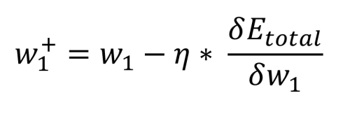
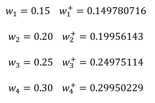
Again, the bias value plays no role in this calculation. Now we can compare the old weights w1 through w4 and the new weights:
With the new weights determined, the old weights can be replaced by the new weights and a new forward pass can be executed. As long as the output error remains larger than desired, backpropagation passes can be repeated as described here.
MLP Implementation in Processing
To demonstrate this simple neural network, a neural network was coded from scratch as a class that can be used in Processing [11], the development environment designed for promoting coding within the visual arts. The visual capabilities of the IDE allow 2D and 3D graphics to be displayed with ease. A text console output also allows ideas to be tested quickly and easily. The code that follows is part of the repository mentioned [10].
The code for the MLP implementation is found in the folder processing/neural/neural.pde. This file simply needs to be added to any Processing project that intends to use it. The Neural class can be instantiated to support any number of input, hidden, and output nodes as desired. To replicate the example already covered, the file processing/nn_test/nn_test.pde should now be opened in Processing.
Creating a neural network is quite simple. Firstly the class constructor Neural (in nn_test.pde) is called to create an object, here named network, defining the desired number of inputs, hidden nodes, and outputs (2, 2, and 2). Once created, further member functions are called to set the learning rate and the biases to the hidden node and the output node, as per the example sketch.
The constructor also initializes the weights with random values between 0.25 and 0.75. To match the example, we change the weights as shown in Listing 1 where the input values and the desired output values are also defined.
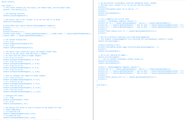
The example code also enables a verbose mode that enables the working for each step of the calculations to be shown. These should match with the results shown in the Excel spreadsheet.
After clicking on Run in Processing, the text console should output the following:
...forwardpass complete. Results:
For i1 = 0.05 and i2 = 0.1
o1 = 0.75136507 (but we want: 0.01 )
o2 = 0.7729285 (but we want: 0.99 )
Total network error is: 0.2983711
After this, ‘learning’ is enabled and a forward pass is executed again followed by the backpropagation step. This results in the output of the new and old weights and the calculation of a new forward pass to determine the new output node values and errors:
New Hidden-To-Output Weight [ 0 ][ 0 ] = 0.3589165, Old Weight = 0.4
New Hidden-To-Output Weight [ 1 ][ 0 ] = 0.40866616, Old Weight = 0.45
New Hidden-To-Output Weight [ 0 ][ 1 ] = 0.5113013, Old Weight = 0.5
New Hidden-To-Output Weight [ 1 ][ 1 ] = 0.56137013, Old Weight = 0.55
New Input-To-Hidden Weight[ 0 ][ 0 ] = 0.14978072, Old Weight = 0.15
New Input-To-Hidden Weight[ 1 ][ 0 ] = 0.19956143, Old Weight = 0.2
New Input-To-Hidden Weight[ 0 ][ 1 ] = 0.24975115, Old Weight = 0.25
New Input-To-Hidden Weight[ 1 ][ 1 ] = 0.2995023, Old Weight = 0.3
We can see that these represent weights 5 through 8 and then 1 through 4. They also match the hand calculations made earlier (with small exceptions due to some rounding error).
Next Steps with MLP and More on Neural Networks
Want to learn more about neural networks? Having developed a good understanding of how an MLP neural network functions and the example Neural class provided here for Processing, the reader is well-positioned to undertake further experimentation independently. Some ideas include:
- Running the learning in a loop — How many epochs are required to achieve a network error of 0.001, 0.0005, or 0.0001?
- Start with different biases and weights - How does this impact the number of epochs required to learn? Does the neural network ever fail to learn?
- Map outputs to inputs - Try generating a 3D plot of each output against the inputs once the network has learned its task. Does it look like you'd expect? You may prefer to try Plotly's Chart-Studio instead of using a spreadsheet [ 12 ] to plot the output data .
In the next article in this series about neural networks, we will teach our neural network how to implement logic gates and visualize its learning process.
Do you have questions or comments regarding neural networks or anything else covered in this article? Then email the author at stuart.cording@elektor.com .
Discussion (0 comments)