
Understanding the Neurons in Neural Networks (Part 2): Logical Neurons
on
In the first part of this article series, we discovered how researchers slowly approximated the functionality of the neuron. The real breakthrough in artificial neurons came about with the multilayer perceptron (MLP) and using backpropagation to teach it how to classify inputs. Using a from-scratch implementation of an MLP in Processing, we also showed how it worked and adjusted its weights to learn. Here we go back to the experiments of the past to teach our neural network how logic gates function and check if our MLP is capable of learning the XOR function.
We have a flexible Neural class to implement an MLP that can be incorporated into any Processing project. But the examples reviewed thus far didn’t achieve very much. They simply confirm the forward pass's correct calculation and how backpropagation adjusts the network’s weights to learn a given task.
Now it is time to apply this knowledge to a real task, the same task investigated during the early studies of the McCulloch-Pitts Threshold Logic Units (TLU): implementing logic. As we already discovered, our MLP should solve linearly separable problems such as AND and OR with ease. Additionally, it should also be able to solve the XOR function, something that the TLU and other early artificial neurons could not. On this journey, we shall also examine how these networks learn thanks to a visual implementation of the neural network. We shall also look at the impact the chosen learning rate has on the output error during learning.
AND
While a neural network can learn to replicate the function of AND, it doesn’t function in quite the same way. What we actually do is apply inputs to a network that has learned the AND function and ask it: “How confident are you that this input combination is the pattern we attribute a 1 to?”
To demonstrate this, an example project has been prepared and is available from the GitHub repository in the folder /processing/and/and.pde. This should be opened using Processing.
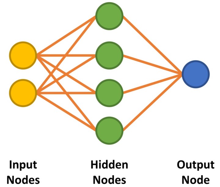
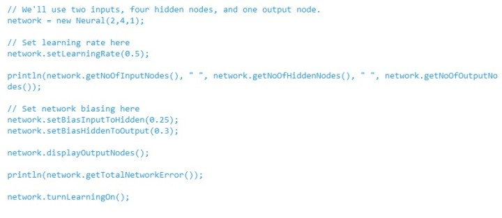
Our neural network has two inputs and a single output to remain true to a two-input AND gate. Between the input and outputs nodes, we implement four hidden nodes (Figure 1). We shall discuss the way to approach determining the number of required hidden nodes later on. The code to prepare the network is shown in Listing 1.
The goal is to train the network to recognize the pattern ‘11’ at the inputs. We also want to be sure that the alternatives ‘00’, ‘01’, and ‘10’ do not exceed our classification threshold. While teaching the network, we shall apply the stimuli and expected results shown in Table 1.
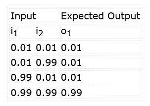
Note that, rather than working with logic levels, such networks work with decimal values. A 1, in this case, is input as 0.99 (almost 1), whereas a 0 is input as 0.01 (almost 0). The output will also range between 0.0 and 1.0. This should be evaluated as a confidence level that the inputs match the classification learned, e.g., 96.7% confidence both inputs are ‘1’, rather than the clear 0/1 logic output of a real AND gate.
We can start by determining if this newly created network ‘knows’ anything by providing it with some inputs and asking it for its output. Remember, the results generated will differ each time as the constructor applies random values to the weights.
The code below outputs the network’s response to ‘11’ and ‘00’ at the inputs. It is highly likely that the result for ‘11’ will be close to 0.99, while the result for ‘00’ will be much larger than the hoped for 0.01:
// Check output of AND function for 00 input
network.setInputNode(0, 0.01);
network.setInputNode(1, 0.01);
network.calculateOutput();
println(“For 00 input, output is: ”, network.getOutputNode(0));
// Check output of AND function for 11 input
network.setInputNode(0, 0.99);
network.setInputNode(1, 0.99);
network.calculateOutput();
println(“For 11 input, output is: ”, network.getOutputNode(0));
This delivered the following output during testing:
For 00 input, output is: 0.7490413
For 11 input, output is: 0.80063045
We see here that when we apply 0.99 to both inputs, the neural network thinks that the input is ‘1 AND 1’ with a confidence of 0.8006, which converts to 80.06%. This is not bad at this stage. However, when applying 0.01 to both inputs, it has a confidence of 0.7490 (74.90%) that the input is ‘1 AND 1’. This is a long way from what we want, which is something close to 0%.
To teach the network how an AND function works, it must be trained. This is achieved by setting the inputs and desired output appropriately for all four cases (00, 01, 10, and 11, and 0, 0, 0, and 1 respectively) and calling the calculateOuput() method with ‘learning’ enabled after each change. This is performed in a loop as follows:
while (/* learning the AND function */) {
// Learn 0 AND 0 = 0
network.setInputNode(0, 0.01);
network.setInputNode(1, 0.01);
network.setOutputNodeDesired(0, 0.01);
network.calculateOutput();
// Learn 0 AND 1 = 0 … Learn 1 AND 0 = 0
// Learn 1 AND 1 = 1
network.setInputNode(0, 0.99);
network.setInputNode(1, 0.99);
network.setOutputNodeDesired(0, 0.99);
network.calculateOutput();
}
network.turnLearningOff();
The decision to stop the training of the network can be determined in a number of ways. Each learning cycle in this example is considered to be an epoch. Learning can be stopped once a specific number of epochs, such as 10,000, is achieved. Alternatively, the error in the output can be used. Once it is below, say, 0.01%, the network could be considered accurate enough for the classification task at hand.
One important point to note is that an MLP does not always converge on the result desired. You may be unlucky due to the combination of weights and bias weights selected. Alternatively, the configuration of the MLP may not be capable of learning your task, likely due to too many or too few hidden nodes. Here there are no rules — the appropriate number of nodes, starting weights, and biases can only be determined by trial and error or experience. For this example, four hidden nodes were chosen as four input states must be learned. It was hoped that each hidden node would learn one state.
It should also be noted that training should occur in batches, i.e., the set of training data should be cycled through from beginning to end repeatedly. If ‘0 AND 0 = 0’ is taught repeatedly for several thousand cycles, the network skews toward this outcome, and it becomes almost impossible to train the remaining data.
With the basic implementation covered, we can now look at the example that trains the network to learn the AND function in more detail. To help show how neural networks learn, the network is visualized in the application during learning and, later, during operation.
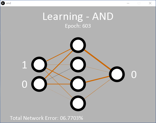
Clicking on ‘Run’ should result in the output shown in Figure 2 (screenshot). Initially the application is in learning mode, teaching the network the expected output for an AND function for the two inputs. On the left are the input nodes. During learning, the input values switch rapidly between the logic levels 0 and 1. On the right is the single output node. Initially, this is 0. The decision to output 1 is made only if the output node delivers a > 90% confidence that both inputs are 1. Otherwise, a 0 is output. This decision is made between lines 341 and 346 in and.pde.
// Output Node Text
if (network.getOutputNode(0) > 0.9) {
text("1", 550, 280);
} else {
text("0", 550, 280);
}
Initially, the output remains 0 as the 90% confidence level has not yet been achieved. After around 5,000 epochs, the output value should start to flicker back and forth between 0 and 1, demonstrating it has begun to successfully classify that the ‘11’ input should output a ‘1’. At this point, the total error of the network is around 0.15%. If this doesn’t happen, it is likely that the network has got stuck and will not be able to learn this time around.
As the network learns, the weights between the nodes are displayed as lines of varying thickness and color. The thicker the line, the larger the value. Black lines indicate positive numbers, while brown lines indicate negative numbers.
Each time the code is executed, the lines will be different. You will, however, notice that a pattern develops. Two hidden nodes always have one brown and one black line; one hidden node has two black lines; and one hidden node has two brown lines. The lines between the hidden nodes and the output node will also conform to a pattern, with the only black line emanating from the node with two incoming black weight lines.
This is an interesting insight as it shows how the network has learned the AND function. ‘00’ at the input converts easily to a 0 at the output, as does ‘11’ into 1. For the ‘01’ and ‘10’ combinations, it seems that the 0s do a lot of the heavy lifting in pushing the output towards 0.
The application is programmed to stop learning once the network's total error is < 0.05% on line 57 in and.pde. Alternatively, the learning can be programmed to stop after a certain number of epochs using line 55. Once learning is complete, the application simply cycles through the binary inputs in order, allowing the neural network to show off what it has learned (Figure 3).
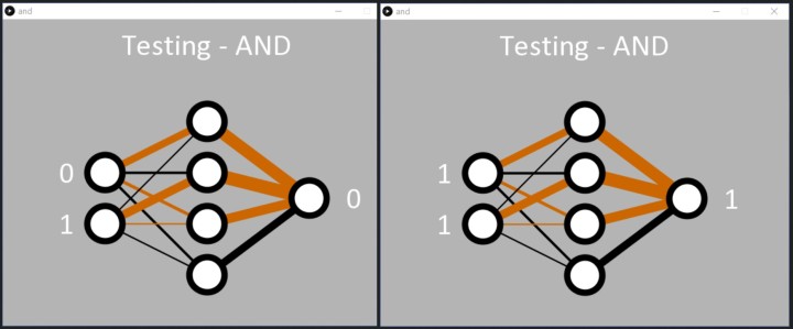
In the text console, the inputs are displayed (as a decimal value between 0 and 3) with the calculated output in text format as follows:
0 : 5.2220514E-4
1 : 0.038120847
2 : 0.04245576
3 : 0.94188505
0 : 5.2220514E-4
1 : 0.038120847
2 : 0.04245576
3 : 0.94188505
For those interested, the output error for the applied inputs and the average network error are written every 50 epochs to a CSV file named and-error.csv. This can be imported into Excel to review how the network converged on the solution (Figure 4). The output shows how the error swings back and forth between high and low values for specific input/output combinations. As we already saw, the high error probably relates to the output for the patterns ‘00’, ‘01’, and ‘10’ being far too high during the early phase of learning. The low error is probably when the network is evaluating the input ‘11’.
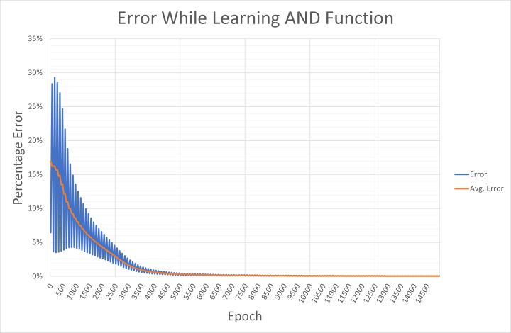
These individual pattern errors are averaged over four epochs to calculate the average network error. Should your PC not use an English locale, you may want to replace the ‘,’ in the CSV file with a ‘;’ as the separator, and then the ‘.’ with ‘,’ in a text editor (such as Notepad++) before performing a data import to Excel.
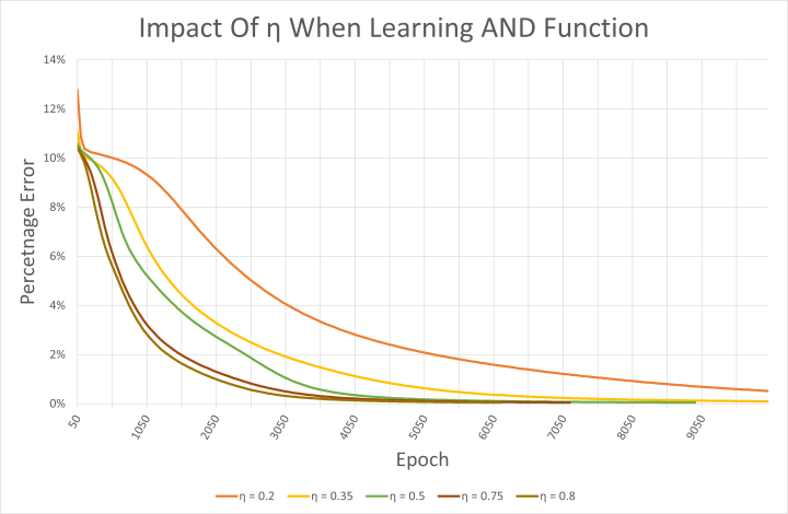
The CSV file is also interesting for reviewing the impact the learning rate has on the network. The example code uses a learning rate η of 0.5. Higher numbers result in the network learning faster, as can be seen in Figure 5. However, they can also cause oscillations and result in a network that never converges on the desired learning outcome. All the learning rates shown trialed here resulted in a correctly functioning network that had learned AND. It should, however, be noted, that the starting weights were randomly chosen each time.
But Can It Learn XOR?
The repository also includes examples for an OR function in processing/or/or.pde. Being linearly separable, the MLP has no trouble learning this function either. The reader may find it useful to examine the difference in the weights after learning compared with the AND example. Both or.pde and and.pde can be easily modified to teach the network the NAND and NOR functions. However, the moment of truth comes with the XOR function.
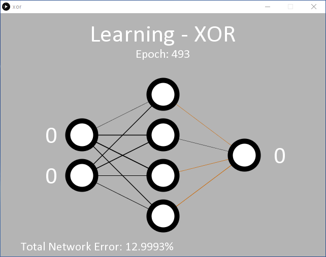
An example for this is provided in processing/xor/xor.pde that operates as the previous code and uses the same 2/4/1 (input/hidden/output) MLP node configuration (Figure 6). At the learning rate used (η = 0.5), it will likely require 15,000 epochs or more before the output starts to change. Around 35,000 epochs are required before the target average error of 0.05% is reached.
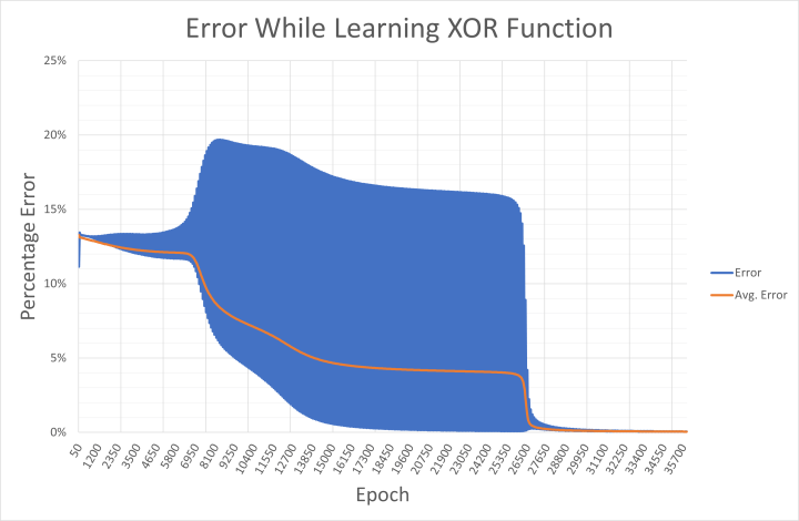
It is clear that the network struggles to learn the XOR function. This is reflected in the displayed weights that flicker between positive and negative before choosing a direction, and the network error drops very gradually. This is because ‘00’ and ‘11’ (represented as 0.01 and 0.01, and 0.99 and 0.99 at the inputs) are both expected to deliver the output 0.01. Mathematically, input values of 0.99 result in high output values until the network is able to push the result down towards 0.01 during learning. This is seen in the output error saved to xor-error.csv during learning (Figure 7).
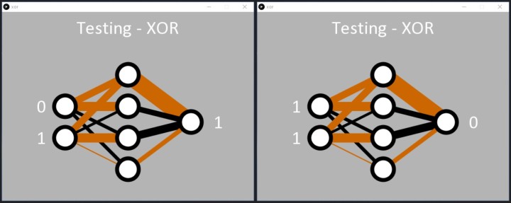
Despite the challenges of the task, the network does learn the XOR function as requested. Once the error is below 0.05%, the Processing code dutifully applies the binary inputs to the network, and the output responds, correctly detecting the patterns ‘01’ and ‘10’. The code then displays a 1 by the output node (Figure 8).
Like with the AND code, we can see how the network has learned the XOR function. Two hidden nodes have a black and brown line entering them and a fat black line leaving them (two middle nodes of Figure 8). These seem to be responsible for the ‘01’ and ‘10’ classification. The network also resolved ‘00’ at the inputs to 0 at the output quite well (top hidden node). On this occasion, the ‘11’ input seems to be handled by the bottom hidden node, but this may not have been resolved very well during learning, resulting in a higher error than desired for the input ‘11’. Rerunning the code will likely result in one hidden node obviously handling the ‘11’ with two black lines entering one of the hidden nodes (Figure 9).
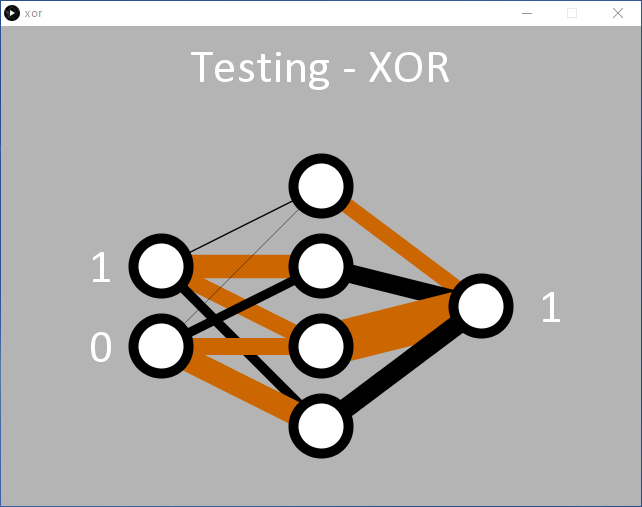
while the third hidden node is responsible for ‘00’.
For Next Time
Perhaps one of the crucial things to take away is that, with neural networks, there is no right or wrong answer. The network itself is merely classifying how likely the inputs you have provided are the inputs you are looking for. If you’ve configured it, trained it, and it delivers the desired result, it is probably correct. Ideally, you are also looking to achieve this with the minimum number of nodes to save memory and calculation time.
While the visualization is nice, it is not totally necessary. If you are interested in discovering more, you may like to modify the processing/fsxor/fsxor.pde project that does away with the visualizations. Removing the code that writes the error values to a CSV file also speeds the code up considerably. You can then write your own code using the Neural class to investigate the following:
- What impact does learning rate have on the network when learning XOR? Perhaps try the same starting weights each time too.
- Can you initialize the weights with values that encourage the network to resolve in fewer epochs? Perhaps review the output weights from an earlier run.
- How few hidden nodes do you need to learn AND? How few to learn XOR? Can you have too many hidden nodes?
- Does it make sense to have two output nodes? One could classify the unwanted patterns as 0.99 (for XOR, ‘00’ and ‘11’), while the second is used to classify the wanted patterns as 0.99 (for XOR, ‘10’ and ’01’).
In the next article on neural networks, we will train the neural network to recognize colors from a webcam attached to our PC. If you like, why not develop and test an MLP node configuration that you think is up to the task?

Questions or comments?
Do you have questions or comments regarding this article? Then email the author at stuart.cording@elektor.com.
Discussion (0 comments)