
Understanding the Neurons in Neural Networks (Part 3): Practical Neurons
on
There have been many predictions regarding self-driving cars [1], none of which have come to fruition. Much of the complexity arises from attempting to understanding the intent of other road users and pedestrians. However, a lot of the autonomous driving system is about classifying everything the many sensors and cameras ‘see’ around the vehicle. This ranges from traffic lights and road signs, to street or road markings, and vehicle types and people. Now that we have a working neural network in the form of our multilayer perceptron, we will use it to detect a traffic light’s colors.
One of the great things about the Processing environment we have used thus far is the ease with which it can access webcams. The examples used here will run on just about any laptop or PC running Windows, Linux or macOS with an integrated or external camera.
Finding Your Camera
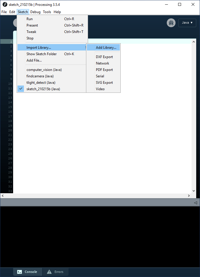
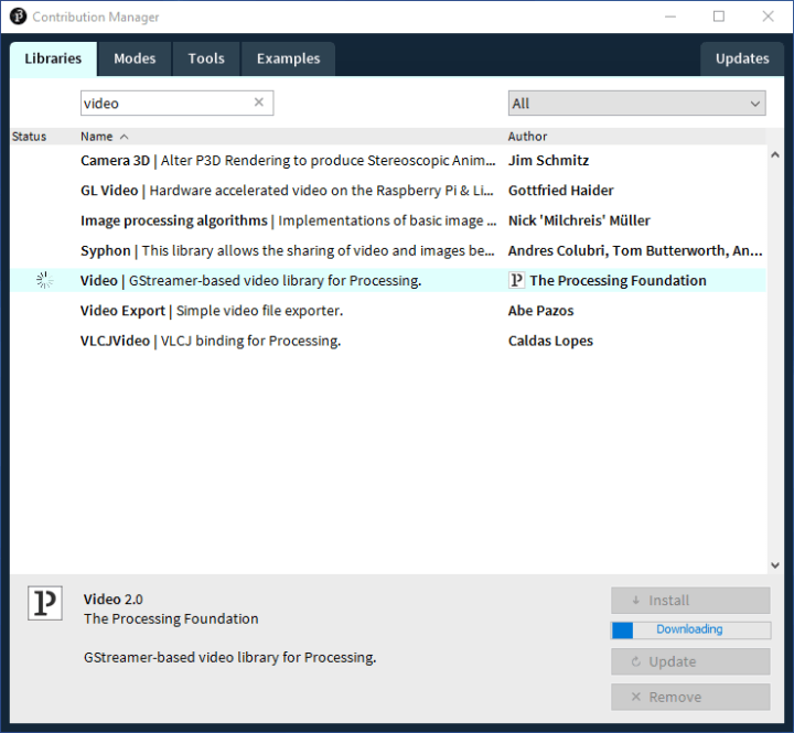
Before we can get started, a new library needs to be added to Processing that provides access to any attached webcams. From the menu, select Sketch -> Import Library… -> Add Library… (Figure 1), which opens the window shown in Figure 2. Ensuring that the Libraries tab is selected, enter “video” into the search box. From the list that appears we select Video | GStreamer-based video library for Processing and then click on Install. As before, we will be using the code from the GitHub repository prepared for this series of articles [2].
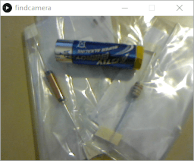
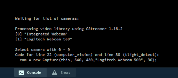
With the library installed, we can run the project /trafficlight/findcamera/findcamera.pde. This code simply requests the list of available cameras connected to the computer and allows the user to select one by entering a number between 0 and 9. Make sure the small findcamera window has the context (click inside the window) before pressing a number. If the Processing IDE window has context, you will simply end up typing a number somewhere in the source code.
Once a camera source has been selected, its output is shown in a low-resolution 320×240-pixel output in the window (Figure 3). The text console will also provide the source code needed to select your camera for the next two projects we will look at (Figure 4).
Finally, we need a traffic light. Since you are unlikely to have one to hand, one has been prepared in trafficlight/resources in various file formats. Simply print one out and keep it to hand.
When stopping Processing projects that use the camera, you may see the message “WARNING: no real random source present!”. This seems to be a bug related to using the Video library but has no impact on the code’s functionality.
How Do Cameras See?
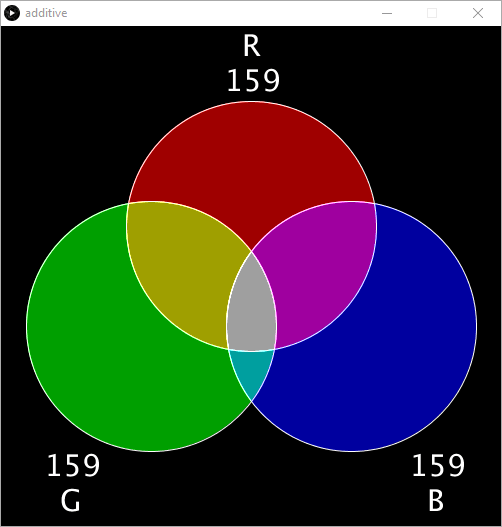
Perhaps one of the most important aspects of using neural networks is to develop an understanding of how a computer can interpret the incoming data. In the case of camera input, the computer image is displayed by mixing the three primary colors, red, green, and blue. This is commonly termed the RGB format. The three values vary between 0 and 255 (or 0x00 and 0xFF in hexadecimal). If we point the camera at something blue, we would expect the B value to be relatively high and the other values quite low. Point it at something yellow, and then there should be a high R and G value as, together, red and green make yellow. To get a better feel for additive color mixing, the project /trafficlights/addititive/additive.pde may be of interest (Figure 5).
With this knowledge, it would seem to make sense to determine how our camera “sees” the colors of our traffic light and note the RGB values it reports. We can then teach our neural network the three traffic light colors so that it may classify them as red, amber, and green.
Determining RGB values
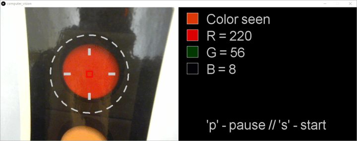
The project trafficlight/computer_vision/computer_vision.pde is the next project we will need. This displays the selected camera’s output next to the RGB values it is reporting. Using this project, we can record the RGB values the camera sees. Before starting the code, don’t forget to paste the line of code you determined in findcamera.pde to line 22 in this project. This ensures your chosen camera is used.
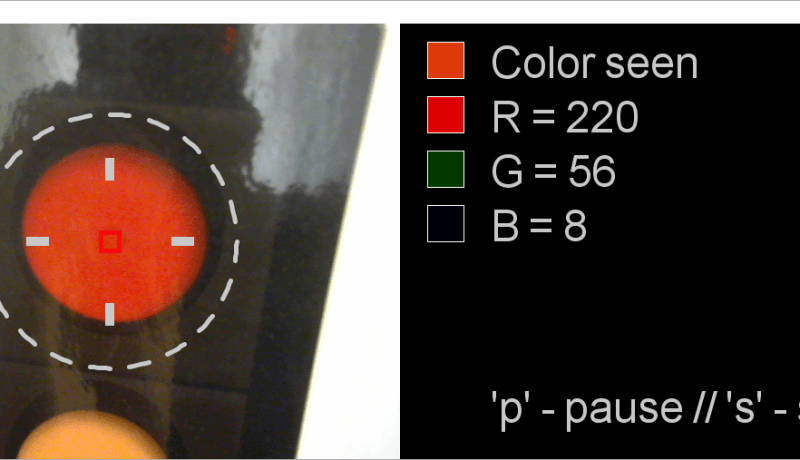
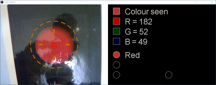
While pointing the camera at the red traffic light (keep the ‘light’ approximately within the dashed circle), note the color seen (top) and the RGB values that define it (Figure 6). The RGB values are actually the average of all the pixels the camera captures in the center’s red bounding square. Despite being an average, the RGB values will change up and down rapidly. To capture a single value, press ‘p’ on your keyboard, and the code pauses on a single set of values. Be sure to click inside this window before pressing ‘p’ to give it the context. Pressing ‘s’ restarts the camera capture and RGB generation again.
The traffic light printout used here was laminated so there are some reflections in places. If you have printed your traffic light image out using a laser printer, you may also have a slightly reflective surface. As a result, although the camera is pointing at the red traffic light, the “Color seen” may be pinkish or even close to white. This is, obviously, not much use for the neural network. It needs to know the color ‘red traffic light’ under optimal conditions, so move the camera or change the lighting until you feel you have achieved an RGB value representing the color optimally.
This also raises another issue concerning accuracy. Drivers will know how difficult it is to discern the active traffic light lamp when the sun is shining into our eyes or directly into the lamps. If we humans cannot distinguish which lamp is lit, how can a neural network figure it out? The answer is, it can’t. If we need a more robust algorithm, we need to train it with ‘poor visibility’ data. We may also need to provide another input, such as where the sun is shining from, so that the neural network knowns when there is ‘poor visibility’ and that it should use the ‘poor visibility’ data set. Finally, we could improve the incoming data from the camera, perhaps by adding an infrared image of the traffic light (which lamps are hot) or some other clever filtering. However, don’t despair! We shall add some robustness into our training data to handle some variation in the color of our traffic light input.
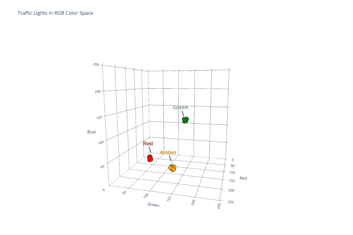
The critical task at this point is to collect the RGB data for the red, amber, and green traffic lights using your camera and your lighting conditions. The data collected using the author’s setup is shown in Table 1.
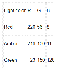
for the three traffic light colors.
Detecting Traffic Lights
Armed with our data, we can now train the neural network the colors of our traffic light. For this final stage we will need the project trafficlight/tlight_detect/tlight_detect.pde open in Processing. Start by ensuring that the correct camera initialization code is pasted into line 38 (from find_camera.pde).
This project uses a three-input, six-hidden, and four-output (3/6/4) node MLP. The three inputs are for the three colors, R, G, and B. Three of the four outputs are to classify the ‘red,’ ‘amber,’ and ‘green’ of the traffic light. The fourth will be used later. The use of six hidden nodes was chosen arbitrarily as ‘enough’ to handle the classification task. We will see that this configuration does work and, as before, readers are encouraged to experiment with fewer or more hidden nodes.
If you run the code ‘as is,’ the neural network operates without any learning. The results (Figure 7) show that any color is classified as all the colors the network is defined to detect.
The teaching of the neural network takes place around line 51. Uncomment the first three methods and add the RGB values you acquired earlier. The three methods used to define red, amber, and green are:
teachRed(159, 65, 37);
teachAmber(213, 141, 40);
teachGreen(128, 152, 130);
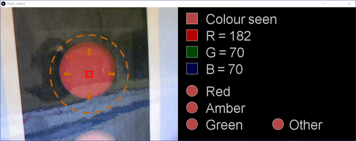
Each time these functions are called, the network is trained to classify that RGB combination as the associated color (Figure 8). To allow for some variation in lighting and automatic changes in exposure setting by the camera, a small amount of variation (±4) to the RGB values is applied using a randomise() function (line 336). Again, you can experiment with the effectiveness of this approach and the amount of randomization applied.
Training of the network is swift compared to previous projects as we are no longer writing the error values during learning to a file. Simply run the project and, after a few seconds, the neural network will start evaluating the color in the red bounding square of the camera window (Figure 9).
The traffic light in the view of the camera is determined on line 156 onwards. The RGB colors captured are applied to the inputs of the MLP and the network’s output is calculated:
network.setInputNode(0, (float) r / 255.0);
network.setInputNode(1, (float) g / 255.0);
network.setInputNode(2, (float) b / 255.0);
network.calculateOutput();
The decision on the color seen is then made starting at line 171. The output of each output node is evaluated. If classification certainty is above 90% (0.90), the color seen is displayed in a circle along with the classifier ‘Red,’ ‘Amber,’ or ‘Green’.
// If likelihood of ‘Red’ > 90%...
if (network.getOutputNode(0) > 0.90) {
fill(200, 200, 200);
// …write “Red”…
text("Red", 640+(100), 320);
// … and set color to the color seen.
fill(r, g, b);
} else {
// Otherwise, set color to black
fill(0, 0, 0);
}
// Now draw the color seen in a circle
ellipse(640+(50), 300, 40, 40);
You can experiment with the accuracy of the MLP by pointing the camera at the different traffic light at different angles and under different lighting conditions. Also, try pointing the camera at objects in your vicinity that, in your opinion, approximate the colors the MLP has learnt.
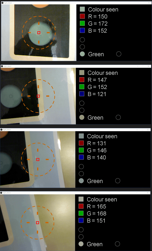
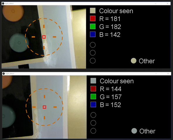
One thing you may notice is the misclassification of a wide range of colors as a known color. In the author’s example, the ‘green’ classification is also given for the traffic light surround, frame, and overall image background (Figure 10).
Tightening-Up Neural Network Classification
From the RGB values displayed, it is clear that the colors passed to the MLP are reasonably close to that of the wanted classification for ‘Green.’ There are several ways to tighten up the classification. The first would be to raise the 90% bar for accurate classification to a higher value. Another may be to increase the number of epochs of learning. The other is to rethink the classification implementation.
So far, we have focused on what we want to positively classify. However, sometimes it can help to teach the neural network what does not belong to the patterns we are looking for. Essentially we can say, “these are three things we are looking for, but here are some similar things we are definitely not looking for.” This is where our fourth output node comes into play.
Returning to the computer_vision.pde project once more, we can capture the RGB values for colors that we want to be classified as ‘other.’ As an example, RGB values for the dark traffic light surround, the white border, and the blue background were collected, with the results as shown in Table 2.
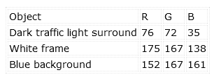
‘unwanted’ colors.
Back in tlight_detect.pde, these values can be taught as ‘Other’ unwanted colors using the teachOther() method. Simply uncomment the code around line 60 as follows and add your RGB values:
teachOther(76, 72, 35);
teachOther(175, 167, 138);
teachOther(152, 167, 161);
Rerunning the project results in a noticeable improvement. The area around the traffic lights (surround, frame, background) is classified as ‘Other’ instead of ‘Green’ (Figure 11).
For Next Time
In this article, we’ve now seen a neural network resolve a real-world classification problem. We’ve also learned that it can help to teach both the desired classification and the undesired classification data.
Why not try building upon this example to explore the following?
- How ‘robust’ can you make the MLP to camera angle and changes in exposure? Is it better to more heavily randomize the learning data or raise the bar for classification (> 90%)?
- Does accuracy improve if you increase the number of ‘Other’ output nodes and teach each one an unwanted color?
- What impact does reducing or increasing the number of hidden nodes have on the system?
- Would a fourth input for ‘general brightness’ help to increase recognition accuracy under varying lighting conditions?
While it is great to run neural networks on powerful laptops and PCs, many of us will desire to have such a capability on the smaller processors used on boards such as Arduino. In our final article of this series, we will use an RGB sensor and an Arduino to implement a color-detecting neural network. Perhaps it will form the basis for your next brainy Arduino project!
Questions About Practical Neurons?
Do you have technical questions or comments regarding this article? Email the author at stuart.cording@elektor.com.
Discussion (0 comments)