The first article of this small series introduced the hardware of the Maixduino and showed how to program it in C++ with the Arduino IDE. The performance of the processor was demonstrated using an artificial intelligence (AI) model for object recognition. How artificial intelligence works in deep learning will be discussed in this installment. If you want to seriously deal with AI, Linux and Python are essential. But with the appropriate tools there is no magic wand.

Please do not expect to have fully grasped Deep Learning after reading the following sections. To do so, I had to study a few books and tutorials as well as numerous programming attempts (and I still don't know much). But I would like to give you at least an overview which structures and methods are used to provide a universally applicable program in the form of a Neural Network (NN) with specialized intelligence.

Structure of a neural network

A neural network (NN) consists of several layers, each of which has several nodes. In Figure1 the nodes of a layer are arranged vertically. Theoretically, there can be any number of nodes per layer and any number of layers in the network. The architecture is determined by the respective task and the size is of course also dependent on the resources of the computer platform used. For example, if the NN is to classify objects that it receives by picture, the first layer takes over the data for solving the task and provides a corresponding number of input nodes for acquisition. If a low-resolution image consists only of 28 * 28 pixels, then 784 nodes are required for a display in grey values. For the acquisition of colour images, the number would triple. During image acquisition, each input node receives the gray value of "its" pixel.

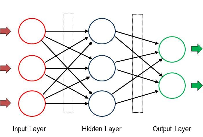
The result of the image analysis is presented in the output layer, which has a separate node for each result. If the NN were to recognize 1000 objects, this layer would have the same number of output nodes. Each node shows a probability between 0 and 1.0 and thus indicates how reliable NN is in the result it has found. For example, when a house cat is taken, the associated node could have a value of 0.85 and the "Tiger" node a value of 0.1. All other nodes would then have even lower probabilities and the result would be unambiguous.

The actual analysis work is done by the hidden layers during deep learning. Depending on the task, any number of hidden layers can be used; in practice, there are certainly 100 to 200 such layers in use. In addition to the architecture shown above, more complex structures with feedback or intermediate filters to increase accuracy can be found. The number of nodes in each hidden layer is also arbitrary. In the above-mentioned example for object detection, three hidden layers with 200 nodes each could already provide useful results.

If in the human brain intelligence is achieved by linking neurons by means of synapses, the nodes in the NN are also networked with each other. Each node of a layer is connected with all nodes of the following layers. Each connection (shown as an arrow in the picture) contains a value called weight. These weights between the layers are stored in matrices. Therefore, in the field of deep learning, programming languages are preferred where matrix operations can be performed easily and quickly.

So how does an NN achieve the desired results? Each node receives its input signals from all nodes of the layer in front of it, marked x in Figure 2.

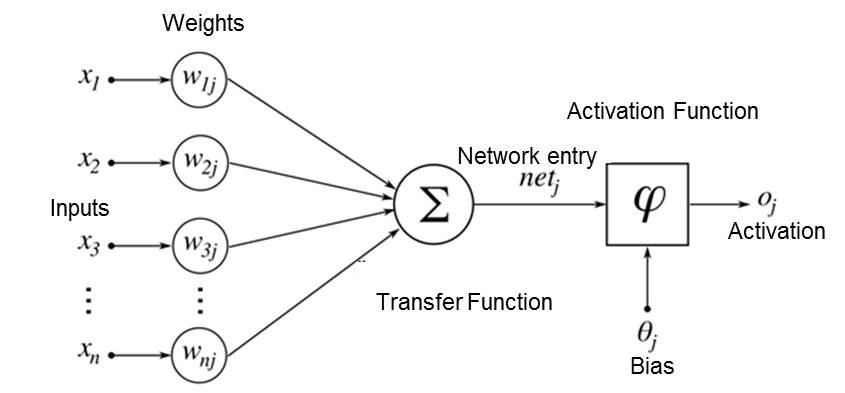
These values are multiplied by the weight values w and added, so the net inputhttp://www.elektormagazine.com/200023-02

net = x1*w1 + x2*w2 + X3*w3 ...

The calculated value of net is now multiplied by an activation function and sent to the output (and thus to all nodes of the subsequent layer). A node-specific threshold value also determines whether this node "fires".

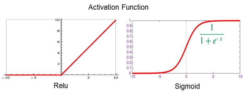
The activation functions shown in Figure 3 are assigned to the layers and ensure that the output values remain within the desired range. For example, the Relu function suppresses all negative values and Sigmoid has a limitation between 0 and 1. These precautions ensure that NNs operate in a clear numerical range and cannot be dominated by " runaways".

Training

So after the input data has been recorded, NN performs numerous calculations in each shift and presents the results at the output. This process is called inference. And how does the intelligence get there? This is done like a small child through education and training. With an untrained NN, the weights are usually filled with random numbers in the value range -1 to +1, so the network is dumb and therefore only provides random results. For training, data and known target output values are fed to the network. After calculation with these values, the result is compared with the setpoint and the difference is documented by a loss function. Now follows the learning process, also called backpropagation. Starting in the last layer, the weights are adjusted in small steps to minimize the loss. After many (often millions of times) of training rounds with different input data, all weights have the values appropriate to the task and NN can now analyze new data unfamiliar to it.

A particularly suitable architecture for image and audio processing is the Convolutional Neural Network, which is also supported by Maixduino. In such a CNN, the neurons (at least in some of the layers) are arranged two-dimensionally, which fits to two-dimensional input data such as an image. Compared to the network indicated in Figure 1, where the activity of a neuron depends on all neurons of the previous layer (via different weighting factors), the dependency is simplified and locally limited in the case of CNN. Here, the activity of a neuron depends only on the values of (for example) 3 x 3 neurons, which are located in the layer before it — the weighting factors are the same. With such a network, small-scale structures such as lines, curves, points and other patterns can be detected particularly well. In the subsequent layers, more complex details and finally whole faces are detected.

In terms of programming, an NN is similar to a spreadsheet, an arrangement of cells with predefined calculation instructions, which access multidimensional matrices with the weights during execution. When classifying new input data, all layers from input to output are passed through and the outputs reflect the respective probability of the result assigned to the node. Well-trained NNs can reach values around 0.9. During training, after the interference, backpropagation takes place with a run from the back to the input to adjust the weights.

Sounds complicated at first, but there are numerous tools and libraries available for the implementation, which I will introduce in the following paragraphs.

Linux and Python

Already in the first article of this miniseries, I pointed out that you have to be prepared for a learning effort when dealing with the topic of artificial intelligence. The easiest way to do it in this world is on the Linux platform, because here most of the tools are available for free and of good quality. Furthermore, Linux offers the same comfort as Windows, but is packaged differently (usually better). My preference is Ubuntu, which is also available as LTS version (Long Term Support) and is supported for at least 4 years. But also the other derivatives like Debian, Mint etc. are just as useful, the choice is a matter of taste. Linux can be installed in a virtual machine besides Windows, for example, so you don't need an extra computer.

And why Python? Python is an interpretive programming language, some will say, so potentially slow. This disadvantage is offset by numerous advantages: Firstly, Python does away with the frills of brackets and semicolons and performs block building by indenting the lines. It has powerful data structures such as lists, tuples, sets and dictionaries; furthermore, Python already has fully integrated matrix calculation. Other major advantages are the available artificial intelligence frameworks and libraries, which can be fully or partially integrated due to their high modularity. These are mostly written in C++ and therefore have the required performance. And all this can be installed easily with just a few instructions.

If you want to get started, please install your favourite Linux as well as pip3 and Python 3, instructions for this are abundantly available on the net.

Maixduino speaks MicroPython

To enable Python to run on systems with less memory, a lightweight version called MicroPython is available; it can be installed on platforms like Maixduino, ESP32 and others. MicroPython contains a balanced repertoire of commands and 55 additional modules for numerous mathematical and system functions. To add new versions or artificial intelligence models, the flashing tool Kflash is required.

Installation of Kflash under Linux:

• Download version 1.5.3 or higher from web link as an archived file kflash_gui_v1.5.3_linux.tar.xz.
• Transfer to a folder of your choice.
• Unpack by command tar xvf kflash_gui_v1.5.3_linux.tar.xz.
• Change to the newly created folder /kflash_gui_v1.5.2_linux/kflash_gui.
• Start with ./kflash_gui (in case of startup problems, check the box Run file as program in the properties of this file).

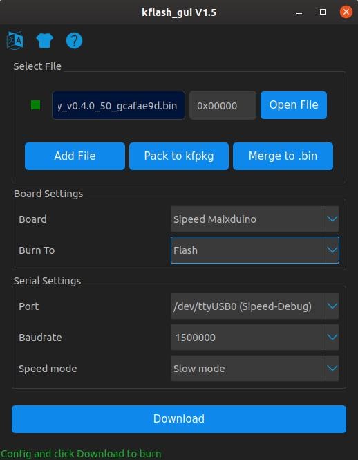
This starts the graphical user interface of Kflash (Figure 4) and you can now load firmware or artificial intelligence models into the Maixduino.

Installing firmware on Maixduino

Even though the Maixduino is already equipped with MicroPython at delivery, you should always download the latest version. When writing these lines, the corresponding firmware is named v0.5.0 and can be downloaded via the web link. Choose maixpy_v0.5.0_8_g9c3b97f or higher and in the next picture choose the variant maixpy_v0.5.0_8_g9c3b97f_minimum_with_ide_support.bin or higher, a file of about 700 kB, which also contains support for the MaixPy-IDE.

With the help of Kflash the new firmware is quickly installed. The Open File button is used to select it and after setting the board, port, baud rate and speed mode as in Figure 5, a click on Download starts the loading process.

After that you can already execute the first Python commands with a terminal emulator (e.g. Putty) via the port /dev/ttyUSB0 on the Maixduino. Here is a small example with array commands:

With libraries like numpy (under Linux) or umatlib even more functions are available.

Installation of MaixPy-IDE

Development and tests are much more comfortable with the development environment called MaixPy-IDE. Python programs can be developed and tested as well as loaded and executed on the Maixduino. Additionally, as shown in Figure 5, tools for image analysis are available. The installation is performed as follows:

• Download the version maixpy-ide-linux-x86_64-0.2.4-installer-archive.7z or higher from web link.
• Transfer to a folder of your choice.
• Unpack by the command tar maixpy-ide-linux-x86_64-0.2.4-installer-archive.7z.
• Change to the new folder maixpy-ide-linux-x86_64-0.2.4-installer-archive and enter the following commands:

./setup.sh

./bin/maixpyide.sh

After that the IDE starts. For subsequent starts, only the latter command is of course required.

Thus, all tools for implementing artificial intelligence models are available. In the following a face recognition is tested.

Face recognized!

An trained artificial intelligence model is used for face recognition, which has already analyzed several thousand faces for characteristic features - the weights of the NN used are adjusted accordingly. The model is available for download under the web link under the name face_model_at_0x300000.kfpkg. The basis of the development is the AI framework Yolo2 (You Only Look Once), which divides the image objects into several zones, analyzes them separately and thereby achieves high recognition rates (I will talk about the artificial intelligence frameworks later in this series). The artificial intelligence model for the AI processor is packed in kfpkg format and must be flashed to address 0x300000 in the Maixduino. This can also be done with Kflash; just find the file using Open File and load it onto the board using the parameters from Figure 4.

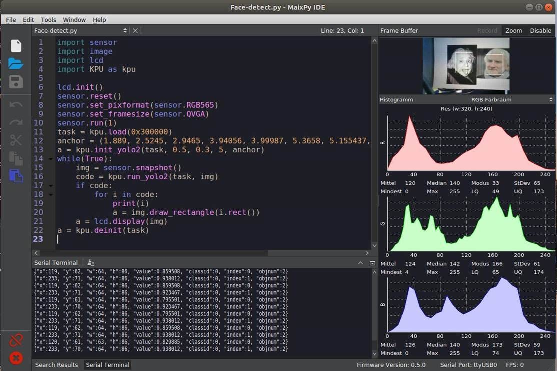
The MaixPy-IDE is used for comfortable handling of the Python script. With this IDE you can develop and test programs and transfer them to Maixduino. Figure 5 shows the interface divided into three windows:

Editor, top left: In this area the program input is done with syntax highlighting.

Terminal, below: Display of the program output.

Image Analysis, right: This is where the display of images and their spectral division into the colours red, green and blue is performed.

Among other available buttons and menu items, the two buttons on the lower left are important: The "paperclip" is used to establish (colour green) or disconnect (red) the connection to the Maixduino via the port "ttyUSB0". A green triangle below it starts the script; then this button changes to a red dot with "x" and serves to stop the program.

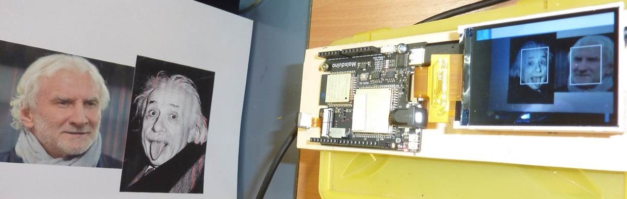
To perform the test, I printed the faces of two publicly known people (Albert Einstein and Rudi Völler) and pinned them to a wall. The selection was purely coincidental, but both faces are said to resemble somewhat, which is not confirmed by me. When taking these pictures, the faces were immediately recognized and marked with a frame. It is important to make sure that the images are displayed in landscape format as shown, otherwise the recognition rate drops noticeably.

The program Face-detect.py can be found in the download folder on the Elektor website. Its brevity again reflects the performance of the libraries used. To start, the required libraries for camera, LCD and KPU are integrated and initialized. After that, the NN is loaded into the KPU starting at address 0x300000. When the AI model is initialized by the command kpu.init_yolo2, additional constants are transferred for setting the accuracy and optimization. Now the image classification is carried out in an endless while loop, an image is taken and fed to the NN. If faces have been detected, the variable i receives for each face the coordinates and size of a marker frame, which is then drawn into the image. Finally, the image (on the LCD panel) and the marking data (on the serial terminal) are output. More details about the KPU commands can be found under the link.

In the MaixPy-IDE the picture is also shown in the upper right corner and the corresponding colour spectrum is displayed below. If you do not need this information, the right image window can be switched off with the deactivate button.

For better handling I mounted Maixduino and LCD on a small board and aligned the camera to the front (see Figure 6). This makes it easy to capture and analyze real faces, printed images or screen contents.

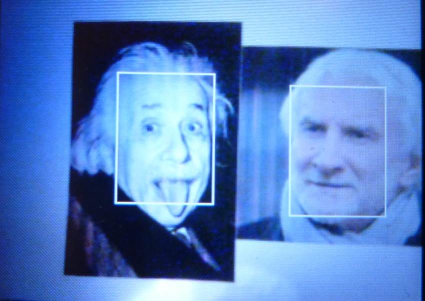
You can see the display on the LCD panel in Figure 7, similarities of the persons are not visible.

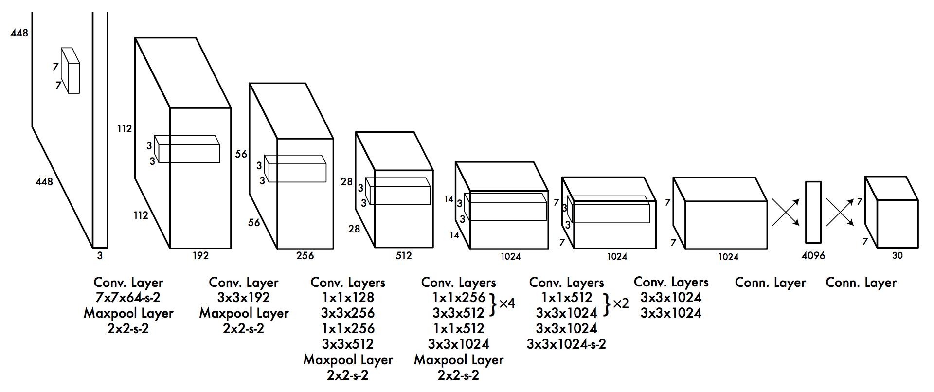
But what is behind this Yolo2 model? The neural network has 24 convolutional layers and two fully connected output layers (see Figure 8). In between there are some maxpool layers as filters to remove complexity and to reduce the tendency to "memorize". It is noticeable that a window size of 3x3 is largely used for detail recognition. Exactly this is supported by the KPU hardware, which ensures that the Maixduino is highly efficient for such tasks.

Other known NN structures even have several hundred layers, have feedback paths or other extras. There are no limits to creativity in this area, much depends on the budget, i.e. computing power.

And on we go!

The powerful hardware and the already available software environment show that the Maixduino is well suited for the entry into Artificial Intelligence. Due to its low power consumption it is well suited for use in mobile devices with already trained neural networks. In a third part of the series I will show you how to develop, train and execute your own neural network. The interface to the developer is the AI framework Keras, which is also known as a comfortable "Lego construction kit for AI". You will also get hints on how to program ESP32 on the board - for example to acquire analogue values.

Stay curious!

Go to Part 1

Want to Learn More About Artificial Intelligence?

Take out an Elektor membership today and never miss an article, project, or tutorial about artificial intelligence.

----------------------------------------------------------------------------------------------------------------------